Week - 2 - Explicit and Implicit Analysis
AIM: The given equation is to be solved by using both Explicit and Implicit Methods ( have a tolerence of 0.001).
Theory:
There are two methods of solving fininte element methods:
- Explicit analysis
- Implicit analysis
Implicit analysis:
Implicit analysis is generally used to solve static problems and Quasi-static problems, uses numerical methods to converge to the theoritical or real solutions. Implicit analysis is Unconditionally stable.
The solving of implicit problems contains the inversion of matrix, If point of interest is at many points the problem is going to get much complex and not economical with more time consumption.
Time step considered in implicit analysis is very large, due to the complexity in solving the problem.
In static problems, we are interested in finding the solution at the point of application of load. Hence, there is no need of finding solutions in between points.
In Quasi-static problems, we are interested in finding the solution at middle and at end of the span. The process is very slow and can be solved using both imlicit and explicit analysis.
Explicit analysis:
Explicit analysis is generally used to solve dynamic and quasi static problems. Explicit analysis is conditionally stable.
Explicit analysis is only a incremental problem which uses the solutions obtained before to get the present solution. The complexity of solving the solution is less and time consumes is very less and economical.
Time step consired in explicit analysis is very small, Solver calculates all of the local finite element variables for given incrementation, and move to the next one. Each increment is calculated extremely fast.
Dynamic problems are the fuctions of time and time step is small.
Summary:
Implict analysis is incremental and iterative, It solves the equation untill the equations of equilibrium are satisfied. Implicit will cause iterations to make sure that the error = 0 or within tolerance limits. if not further iterations are carried out.
Where as in explicit analysis, only incremental analysis takes place which do not care if equilibrium equations are satisfied or not. That is reason why explicit analysis takes much less time and more economical than Implicit analysis.
When dynamic events happen slowly in comparison to wave propagation speeds then typically implicit solvers are best. When dynamic events happen on the order of wave propagation speeds then explicit solvers are probably best.
Impact and explosives are better solved explicitly. Typically mechanically applied loads are more implicit.
Explanation:
Given,
F(u) = u3+9u2+4u
k(u) = (dF/du) = 3u2+18u+4
Explicit Analysis
if the nonlinear force versus displacement relationship is not known, but the stiffffness is known, it is possible to construct the graph of force versusdisplacement numerically. One method is to use an incremental explicit load control scheme.
For this example three equal load increments (or steps) of ∆F = 1unit each are used to load the tension bar. The variables used are u for displacement, f for internal force in the bar, F for external force applied to the bar and k for stiffffness. Incremental displacements or incremental externally applied forces are represented as ∆u or ∆F,respectively. Use is made of the relationship ∆F = k∆u.
STEP 1:
The initial conditions:
Force at u=0 is zero. [ F(0) = 0 ], ∆F = 1
Stiffness at u=0 is 4. [K(0) = 4]
∆u1 = ∆F / k(u0) = 1/4 = 0.25.
u1= u0 + ∆u1 == > u1 = 0+0.25 = 0.25
f(u1) = 1.578125
Step 2
⇒ k(u1) = 8.6875
∆F= 1,
∆u2 = ∆F/k(u1) = 1/8.6875 = 0.115107913
u2= u1+ ∆u2 = 0.25 + 0.115107913 = 0.365107913
f(u2) = 2.708836
Step 3
⇒ k(u2) = 10.97185381
∆F= 1,
∆u2 = ∆F/k(u2) = 1/10.97185381 = 0.0911423
u3= u2+ ∆u2 = 0.365107913 + 0.0911423 = 0.456250213.
f(u3) = 3.79345415
Fext = ∆F + ∆F + ∆F = 3.0
It is evident from the results that external and internal forces are NOT in equilibrium because F external is not equal to F internal.
Table 1 summarizes the main results for the explicit analysis:
|
Step i |
∆Fi |
∆ui |
ui |
(F ext)i |
(f int)i |
f int − F ext = R |
| 1 | 1 | 0.25 | 0.25 | 1 | 1.578125 | 0.578125 |
| 2 | 1 | 0.1151 | 0.3651 | 2 | 2.708836 | 0.708836 |
| 3 | 1 | 0.09114 | 0.45625 | 3 | 3.79345415 | 0.793454 |
Implicit Analysis:
An implicit analysis is the same as the explicit analysis, except that at the end of each step.Newton-Raphson iterations are used to enforce equilibrium before moving to the next step.Basically, an incremental force is applied to advance the solution forward at the beginningof a step. However, internal forces and external forces will not be in equilibrium unless thestiffffness is linear for the given step. Hence, in order to achieve equilibrium, corrections mustbe made to the displacement. This is accomplished by using Newton-Raphson iterations tominimize the residual, R(u) = f int − F ext.
Expanding the residual as a Taylor series about the current displacement uj gives
R j+1 = R j (u j ) + (dR(uj )/du)δuj+1 + ... = Rj + k(uj )δu(j+1) + .........
By neglecting higher order terms in the series, setting Rj+1 = 0 and solving for δuj+1 the following correction is obtained
δuj+1 = (−[k(uj )]^−1)*Rj.
here j is representing the number of interation.
Notice that the iteration variable is j and it may take several iterations for the norm of the residual, k Rk , to be reduced below the chosen tolerance criteria. The implicit analysis proceeds as follows (results are approximate, they are more precise if done in a computer to machine precision).
Given, To maintain the tolerance value of 0.001
Step 1:
initial condition: u(0) = 0, ∆F = 1, Fext = 1.
⇒ K(0) = 4
∆u1 = ∆F/k(u0) = 1/4 = 0.25
u1 = uo + ∆u1 = 0.25
f(u1) = f(0.25) = 1.578
k(u1) = k(0.25) = 8.6875
R = F internal - F external
R1 = 0.578125
As R1 > 0.001 Newton Rapson iterations are necessary.
1st Iteration:
δu 11 = -(8.6875)^(-1) * 0.578125
= -0.066546
U corrected = u1 + δu 11 = 0.25-0.066546 = 0.183453
f(U corrected) = 1.042883
k(U corrected) = 7.40312
Residue 1 = 1.042883-1 = 0.042883
As R1 > 0.001 Newton Rapson iterations are necessary.
2nd Iteration:
δu21 = δu(1) − ([k(u (1) 1 )]^(−1) ) *R(1) = -0.066546 - [(1/7.403124)*0.042883] = -0.07234
U corrected = 0.25-0.07234 = 0.17766
f(U corrected) = 1.000315
Residue 2 = 1.000315-1 = 0.000315
Given tolerence of 0.001 is maintained.
no further iterations are necessary.
Therefore, the final value is u1 = u21 = 0.17766.
Step 2:
initial condition: u1 = 0.17766, ∆F = 1, Fext = 2.
⇒ K(u1) = 7.29257
∆u2 = ∆F/k(u1) = 1/7.29257 = 0.13713
u02 = u1 + ∆u2 = 0.17766+0.13713 = 0.31479
f(u2) = 2.18219
k(u2) = 9.9635
R = F internal - F external
R0 = 2.18219-2 = 0.18219
As R0 > 0.001 Newton Rapson iterations are necessary.
1st Iteration:
δu 1 = -(9.9635)^(-1) * 0.18219
= -0.01829
U21 corrected = u20 + δu 1 = 0.31479-0.01829 = 0.2965
f(U21 corrected) = 2.00328
k(U21 corrected) = 9.60074
Residue 1 = 2.00328-2 = 0.00328
As R1 > 0.001 Newton Rapson iterations are necessary.
2nd Iteration:
δu21 = δu(1) − ([k(u (1) 1 )]^(−1) ) *R(1) = -0.01829 - [(1/9.60074)*0.00328] = -0.01863.
U22 corrected = 0.31479-0.01863 = 0.29616.
f(U22 corrected) = 2.00001
k(U22 corrected) = 9.59401
Residue 2 = 2.00001-2 = 0.00001
Given tolerence of 0.001 is maintained.
no further iterations are necessary.
Therefore, the final value is u2 = 0.29616
Step 3:
initial condition: u2 = 0.29616, ∆F = 1, Fext = 3.
⇒ K(u2) = 9.59401
∆u3 = ∆F/k(u2) = 1/9.59401 = 0.10423
u03 = u2 + ∆u3 = 0.29616+0.10423 = 0.40039
f(u3) = 3.10856
k(u3) = 11.68796
R = F internal - F external
R0 = 3.10856-3 = 0.10856
As R0 > 0.001 Newton Rapson iterations are necessary.
1st Iteration:
δu 3 = -(11.68796)^(-1) * 0.10856
= -0.00929
U13 corrected = u03 + δu 3 = 0.40039-0.00929 = 0.39110
f(U13 corrected) = 3.00086
Residue 1 = 3.00086-3 = 0.00086
Given tolerence of 0.001 is maintained.
no further iterations are necessary.
Therefore, the final value is u3 = 0.3911
Results plot:
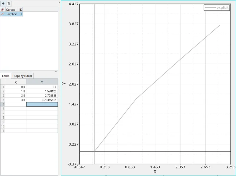
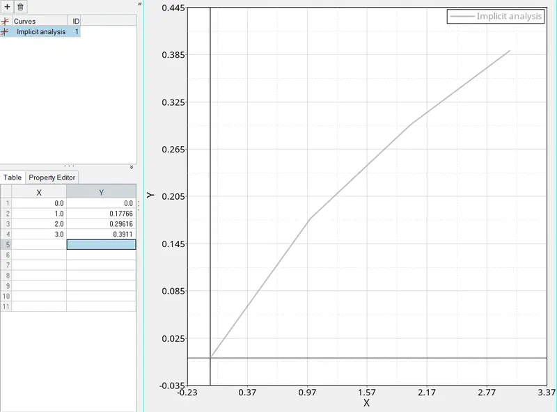
We can observe the values are almost coinciding with error in explicit is less than 10% of the implicit results.
The explicit method is the handy method for the complex models by using a small time step.
Conclusion:
The Implicit and explicit numerical analysis is carried out from the given equation.
From the graphs, we can see the implicit results are more accurate but time consuming and complex for complex applications like crash analysis.
Where as Explicit results are deviating less than 10% from the exact results and is very less time consumable and economical.