Week - 2 - Explicit and Implicit Analysis

Aim:

To briefly explain the implicit and explicit solver methods, and to solve the given polynomial equation using both the methods and compare the differences in the solver method.

Introduction:

All engineering simulation problems involve solving differential equations that involve unknown derivatives, and solving exact solutions will be unavailable, hence numerical methods such as implicit and Explicit methods are used for obtaining the numerical solutions for time-dependent ordinary and partial differential equations (ODE AND PED) by using these methods one can find approximate solution compared to the exact solution.

Explicit and Implicit Methods

Implicit method: In this method, dependent variables are related by coupled set of equations, i.e., solving an equation involving current state of system and the later one to find the solution, uses matrix or iterative technique to obtain the solution. This method has no limit on the size of time step. Implicit method checks for convergence after every time-step this is achieved by incorporating a correction scheme using newton Raphson iteration to minimize the residual This method is suitable for highly linear problems.

Explicit method: Explicit methods use the solutions of the system at the current time to calculate the solution of a system at a later time. In this method, a time step is chosen and this time step determines the accuracy of the approximate solution and number of computations, as the time step size decreases the inaccuracy between the approximate and exact reduces and vice versa, reducing the time step increases the amount of computation and time, due to this it is considered as a conditionally stable method. This method is suitable for dynamic non-linear analysis such as high velocity impact like crash test.

Calculation of the equation in Explicit method:

Equation: `f(u) =(u)^3 + 9(u)^2 + 4u`to solve this equation an incremental explicit load control scheme is used. Three equal load increment of ∆F = 1 unit are used, u is displacement f is internal force, f is external force applied, K is stiffness ,incremental displacement and externally applied load are ∆u and ∆F.

Force(F) = Stiffness (K)* displacement (u)

Stiffness `K(u)=(deltaf(u))/(delta(u)) = 3u^2 + 18u + 4 = 3u^2 + 18u + 4`

Step1:

First load-increment = `DeltaF=1`

`u_0= 0 Rightarrow k(u_0)= 3(u_0)^2 + 18u_0 + 4 = 3*0^2+18*0+4=4`

`Deltau_1= (DeltaF)/(k(u_0))= 1/4=0.250`

`u_1 = u_0 + Deltau_1=0+0.25=0.250`

`f(u_1) =(u_1)^3 + 9(u_1)^2 + 4u_1 Rightarrow (0.25)^3 + 9(0.25)^2 + 4(0.25)= 1.578`

`Residual (R_1) = f_1-DeltaF_1 = 1.5781-1=0.578`

Step 2:

second load-increment = `DeltaF=1`

`u_1= 0.25 Rightarrow k(u_1)= 3(u_1)^2 + 18u_1 + 4 = 3*0.25^2+18*0.25+4=8.687`

`Deltau_2= (DeltaF)/(k(u_1))= 1/8.6875=0.115`

`u_2 = u_1 + Deltau_2=0.250+0.115=0.365`

`f(u_2) =(u_2)^3 + 9(u_2)^2 + 4u_2 Rightarrow (0.365)^3 + 9(0.365)^2 + 4(0.365)=2.709`

`Residual (R_2) = f_2-DeltaF_2 = 2.709-(1+1)=0.709`

Step 2:

third load-increment = `DeltaF=1`

`u_2= 0.365 Rightarrow k(u_2)= 3(u_2)^2 + 18u_2 + 4 = 3*0.365^2+18*0.365+4=10.972`

`Deltau_3= (DeltaF)/(k(u_2))= 1/10.972=0.091`

`u_3 = u_2 + Deltau_3=0.365+0.091=0.456`

`f(u_3) =(u_3)^3 + 9(u_3)^2 + 4u_3 Rightarrow (0.456)^3 + 9(0.456)^2 + 4(0.456)=3.793`

`Residual (R_3) = f_3-DeltaF_3 =3.793-(1+1+1)=0.793`

Step i	`DeltaF_i`	`Deltau_i`	`u_i`	`(F_(ext))_(i)`	`(f_(i nt))_i`	`R=f_(ext)-F_(i nt)`
1	1	0.25	0.25	1	1.578	0.578
2	1	0.115	0.365	2	2.709	0.709
3	1	0.091	0.456	3	3.793	0.793

Calculation of the equation in Implicit method:

Tolerance for the residual, R, to be reduced below 0.001 `(R <10^-2)`

`f(u) =(u)^3 + 9(u)^2 + 4u`

Stiffness `K(u)=(deltaf(u))/(delta(u)) = 3u^2 + 18u + 4 = 3u^2 + 18u + 4`

Step1:

First load-increment = `DeltaF=1`

`u_0= 0 Rightarrow k(u_0)= 3(u_0)^2 + 18u_0 + 4 = 3*0^2+18*0+4=4`

`Deltau_1= (DeltaF)/(k(u_0))= 1/4=0.250`

`u_1 = u_0 + Deltau_1=0+0.25=0.250`

`f(u_1) =(u_1)^3 + 9(u_1)^2 + 4u_1 Rightarrow (0.25)^3 + 9(0.25)^2 + 4(0.25)= 1.578`

`Residual (R^0) = f_1-DeltaF_1 = 1.5781-1=0.578`

`norm(R^0)>10^-2`

Newton-Raphson iterations are necessary to obtain correction factor to bring the R within the tolerance value.

`u_1^((0)) = u_1= 0.25`

`K(u_1^(0))=k(u_1)= 3*0.25^2+18*0.25+4=8.688`

`delta u^((1)) = −[k(u_1^ ((0)) )]^(−1)R^((0)) = -[8.688]^(-1)*0.578 = -0.06653`

Updated = `u_1^((1)) = u_1^(0) + delta u^((1)) = 0.25 + (-0.06653) = 0.183`

to Check the Residual `F_e=1`

`f_(i nt) = (u_1^(1))^3+9(u_1^(1))^2+4(u_1^(1)) = 0.183^3 +9*(0.183^2)+4*0.183 = 1.039`

`R^((1)) = f_(i nt)-F_(ext) = 1.039-1 = 0.039`

`norm(R^0)>10^-2`

2nd iteration:

`u_1=u_1^((0))`

`k(u_1^ ((1))) =3*0.183^2+18*0.183+4=7.394`

`delta u^((2)) = delta u^((1))−[k(u_1^ ((1)) )]^(−1)R^((1)) = -0.06653 -[7.394]^(-1)*0.039 = -0.0718`

`u_1^((2)) = u_1 + delta u^((2)) = 0.25 + (-0.0718) = 0.178`

`f_(i nt) = (u_1^(2))^3+9(u_1^(2))^2+4(u_1^(2)) = 0.178^3 +9*(0.178^2)+4*0.178 = 1.004`

`R^((2)) = f_(i nt)-F_(ext) = 1.004-1 = 0.004`

`norm(R^0)<10^-2`

Satisfies the condition of tolerance, no more iterations necessary.

The final value of `u_2=u_2^(1)=0.178`

The Final value of `f_1=1.004`

Step 2:

Second load-increment = `DeltaF=1`

`u_1= 0.178 Rightarrow k(u_1)= 3(u_1)^2 + 18u_1 + 4 = 3*0.178^2+18*0.178+4=7.302`

`Deltau_2= (DeltaF)/(k(u_1))= 1/7.302=0.137`

`u_2 = u_1 + Deltau_2=0.178+0.137=0.315`

`f(u_2) =(u_2)^3 + 9(u_2)^2 + 4u_2 Rightarrow (0.315)^3 + 9(0.315)^2 + 4(0.315)= 2.184`

`Residual (R^0) = f_2-DeltaF_2= 2.184-2=0.184`

`norm(R^0)>10^-2`

Newton-Raphson iterations are necessary to obtain correction factor to bring the R within the tolerance value.

Iteration 1:

`u_2=u_2^(0)`

`K(u_2^(0))= 3*0.315^2+18*0.315+4=9.967`

`delta u^((1)) = −[k(u_1^ ((0)) )]^(−1)R^((0)) = -[9.967]^(-1)*0.184 = -0.018`

Updated = `u_2^((1)) = u_2^(0) + delta u^((1)) = 0.315 + (-0.018) = 0.296`

To check the residual `F_e=1`

`f_(i nt) = (u_2^(1))^3+9(u_2^(1))^2+4(u_2^(1)) = 0.296^3 +9*(0.296^2)+4*0.296 = 1.998`

`R^((1)) = f_(i nt)-F_(ext) = 1.998-2 = -0.002`

Satisfies the condition of tolerance, no more iterations necessary.

The final value of `u_2=u_2^(1)=0.296`

The Final value of `f_1=1.998`

Step 3:

Third load-increment = `DeltaF=1`

`u_2= 0.296 Rightarrow k(u_2)= 3(u_2)^2 + 18u_2 + 4 = 3*0.296^2+18*0.296+4=9.59`

`Deltau_3= (DeltaF)/(k(u_2))= 1/9.59=0.104`

`u_3 = u_2 + Deltau_3=0.296+0.104=0.4`

`f(u_3) =(u_3)^3 + 9(u_3)^2 + 4u_3 Rightarrow (0.4)^3 + 9(0.4)^2 + 4(0.4)= 3.104`

`Residual (R^0) = f_3-DeltaF_3= 3.104-3=0.104`

`norm(R^0)>10^-2`

Newton-Raphson iterations are necessary to obtain correction factor to bring the R within the tolerance value.

Iteration 1:

`u_3=u_3^(0)`

`K(u_3^(0))= 3*0.4^2+18*0.4+4=11.680`

`delta u^((1)) = −[k(u_3^ ((0)) )]^(−1)R^((0)) = -[11.680]^(-1)*0.104 = -0.008`

Updated = `u_3^((1)) = u_3^(0) + delta u^((1)) = 0.4 + (-0.008) = 0.3911`

To check the residual `F_e=1`

`f_(i nt) = (u_3^(1))^3+9(u_3^(1))^2+4(u_3^(1)) = 0.3911^3 +9*(0.3911^2)+4*0.3911 = 3.0008`

`R^((1)) = f_(i nt)-F_(ext) = 3.0008-3 = 0.0008`

Satisfies the condition of tolerance, no more iterations necessary.

The final value of `u_3=u_3^(1)=0.391`

The Final value of `f_3=3.0008`

Step i	`DeltaF_i`	`u_i`	`(F_(ext))_i`	`(f_(i nt))_i`	`R=f_(ext)-F_(i nt)`
1	1	0.178	1	1.004	0.004
2	1	0.296	2	1.998	-0.002
3	1	0.391	3	3.0008	0.0008

Results and Discussion:

Steps	Force	Explicit `u_i`	Implicit `u_i`	Exact `u_i`
1	1	0.25	0.178	0.177
2	2	0.365	0.296	0.296
3	3	0.456	0.391	0.391

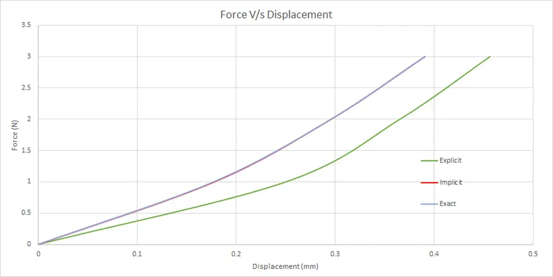
The graph shows that the implicit curve fits well with the exact solution on the other hand the explicit curve deviates from the exact solution, this shows that the implicit method has less error compared to the explicit method, but the solution involves the inversion of stiffness, in FEA as the nodes increase the size of stiffness matrix increases inversion of [K] matrix is computationally heavy and takes more time to arrive at an approximate solution, hence the explicit method is preferred for dynamic non-linear analysis problems. The explicit method can predict approximate solutions to problems much faster than implicit methods, which is important for industries to reduce the design time.

Conclusion:

Mathematical comparison between implicit and explicit numerical methods is carried out by solving the given equation and differences between both methods is drawn in the report.