Week - 2 - Explicit and Implicit Analysis

Aim: To solve this equation, F(u) = u3+9u2+4u using both Explicit and Implicit Methods ( have a tolerence of 0.001).

F = Force ; u = displacement

Overview :

The problem is solved by both an explicit and implicit analysis. In both cases an incremental load control scheme is used.

Ways to solve FE problem--

1. Explicit method:

In explicit, method is stable only when time step is (delta-t) is very small, and equation need not to converge in each time increment. In software time step is decided using below equation

Δt<L√ρ(1−2v)/2μ(1−v) ; μ = shear modulas.

example : To solve this equation using explicit

M (d^2 u)/dt^2 + Ku = F(t)

At t = 0;

we know; u and v and using them we compute M & K.

and then use them to compute acceleration from which velocity & displacement can be calculated at Δt.

a = M^(-1) (F(t)-Ku) ;

v(Δt) = v(0) + a Δt ;

u(Δt) = u(0) + v(0)Δt +1/2 a Δt^2 ;

All the parameters in expicit are taken from the previous time steps

u(n+1) = u(n) + Δt. F(u(n)) ; n = previous time step n+1 = next time step.

Computaion required is less in explicit case as compared to implicit.

2. Implicit method :

In this case long time steps can be given and each time solution need to be converge. It requires more computing power.

To solve above example we only compute M & K at Δt, not at t = 0, and next proceed as above.

u(n+1) = u(n) + Δt. F(u(n+1))

Exlicit Analysis:

Clearly it is possible to plot a graph of force, f, versus displacement, u, by using equation F(u) = u3+9u2+4u. However, if the nonlinear force versus displacement relationship is not known, but the stiffness is known, it is possible to construct the graph of force versus
displacement numerically. One method is to use an incremental explicit load control scheme. This is illustrated next. For this example three equal load increments (or steps) of ▲F = 1 unit each are used to load the tension bar.

K = dF/du = 3u^2 + 18 u + 4

Step 1 :

U(0) = 0; K(u(0)) = 4 , ▲F = 1 , ▲u1 = ▲F/ K(u(0)) = ¼ = 0.25

u1 = u(0) + ▲u1 = .25

f(ini) = .25^3 + 9*.25^2 + 4*.25 = 1.578

R = – ▲F = .578

Step 2:

k(u1) = 3(u1^2) + 18*u1 + 4 = 3*(.25^2) + 18*.25 + 4 = 8.6875

▲F = 1+1= 2

▲u2 = ▲F/k(u1) = 1/8.6875 = .1151

u2 = u1 + ▲u2 = .3651

f(ini) = .3651^3 + 9*.3651^2 + 4*.3651 = 2.709

R = f(ini) – ▲F = .709

Step 3:

▲F = 3

K(u2) = 3(u2^2) + 18*u2 + 4 = 3*(.3651^2) + 18*.3651 + 4 = 10.9717

▲u3 = ▲F/k(u2) = 1/10.9717 = 0.09114

u3 = u2 + ▲u3 = .45624

f(ini) = .45624^3 + 9*.45624^2 + 4*.45624 = 3.79293

R = – ▲F = .79293

Fext ≠ f(ini)

i	▲F(i)	▲u(i)	u(i)	Fext	F(ini)	R
1	1	.25	.25	1	1.578	.578
2	1	.1151	.3651	2	2.709	.709
3	1	.09114	.45624	3	3.79293	.79293

Implicit Analysis:

Plot:

From the plot it is clear that explicit solution drifts away from the exact solutioin as internal force is not equal to external one i.e. there is lack of equilibrium and implicit is giving good results almost exact as force are almost equal and equilibrium is achieved. Only three Newton_rapson iterations are required to get the exact result.

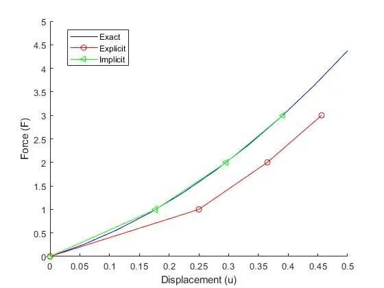
Conclusion: From the plot it is clear that explicit solution drifts away from the exact solutioin and implicit is giving good results almost exact. We can use both methods to solve the problem, however explicit took less time and time interval should be very small for it. But for the implicit we can increase the size of time interval and get the accurate results, but computation and time required will be high. So it depends upon the problem which method to use.