Week 2 Air standard Cycle
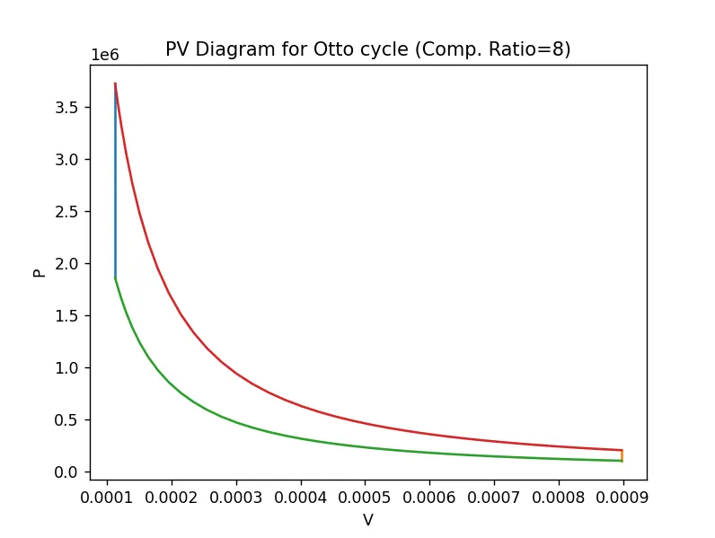
Objective: To plot the ‘PV’ diagram an SI engine running the ideal Otto cycle.
Explanation and process:
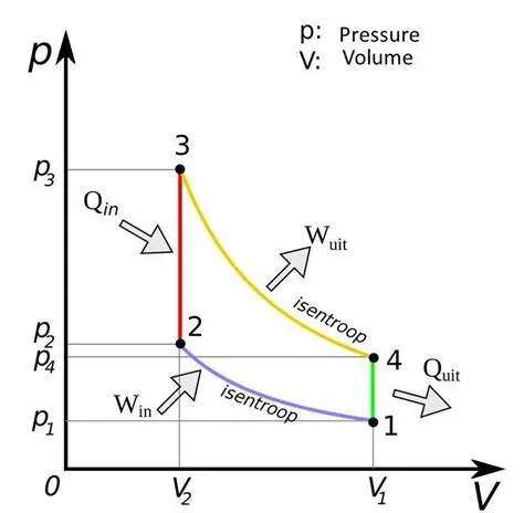
At ‘1’, the air has been sucked into the cylinder. The entire volume of the cylinder (swept volume and clearance volume) is available for the gas.
The process from ‘1’ to ‘2’ is an isentropic compression process (`PV^gamma=constant`). The available cylinder volume at ‘2’ is equal to the clearance volume. The air-fuel mixture becomes combustible once this compression has taken place.
The process from 2 to 3 is the isochoric heat addition process. The spark from the spark plug sets of the combustible mix that causes the rapid expansion of gases.
The process from 3 to 4 is the isentropic expansion process. This constitutes the power stroke. The volume of the available cylinder volume at ‘4’ is equal to the sum of the swept volume and the clearance volume.
The process from 4 to 6 is the isochoric heat rejection process.
The volume during processes ‘1’ to ‘2’ and ‘3’ to ‘4’ varies according to the crank angle “`theta`” which takes on the values "0" to "`pi`" for the process from '1' to '2' and "`pi`" to "0" for the process from '3' to '4'.
This relationship is described by:
`V/V_c=1+0.5*(cr-1)*(R+1-cos(theta)-(R^2-sin^2(theta))^0.5)`
Here,
V->Volume
`V_c` -> Clearance Volume
Cr->Compression Ratio
R->(length of connecting rod)/(0.5*stroke)
The thermal efficiency of the Otto cycle is given by:
`eta=1-1/(cr^(gamma-1))`
Where ‘`gamma`’ is the ratio of the specific heat of air at constant pressure to the specific heat at constant volume.
A code was then written in python to plot the resulting 'PV' diagram.
The code:(with comments explaining each step)
import math
import numpy as np
import matplotlib.pyplot as plt
def volEng(bore,stroke,conRod,cr,start_crank,end_crank,div):
a=stroke*0.5
R=conRod/a
v_s=math.pi/4*bore*bore*stroke #Swept volume of piston
v_c=v_s/(cr-1) #Clearance volume
# theta=math.radians(0)
sc=math.radians(start_crank)
ec=math.radians(end_crank)
theta_ndarray=np.linspace(sc,ec,div)
theta=theta_ndarray.tolist()
v=[]
for t in theta:
term1=0.5*(cr-1)
term2=R+1-math.cos(t)
term3_temp=pow(R,2)-pow(math.sin(t),2)
term3=pow(term3_temp,0.5)
vol=(1+term1*(term2-term3))*v_c
v.append(vol)
return v
#Engine parameters:
bore=0.1
stroke=0.1
conRod=0.15
gamma=1.4 #For air
v_s=math.pi/4*bore*bore*stroke #Swept volume of piston
cr=8
v_c=v_s/(cr-1) #Clearance volume
#inputs:
p1=101325
t1=500
v1=v_c+v_s
rhs=p1*v1/t1 #as it is a closed system, 'pv/t' will be constant throughout...
t3=2300 #Combution temperatures
div=50
#Point 2; (1->2 is an isentropic compression process)
v2=v_c
p2=p1*pow(v1,gamma)/pow(v2,gamma) #isentropic relationship
t2=(p2*v2)/rhs
#Point 3; (2->3 is an isochoric process of heat addition)
v3=v2
#t3 is already defined as the combution temp...
p3=rhs*t3/v3
#Point 4; (3->4 is an isentropic process of expansion)
v4=v1
p4=p3*pow(v3,gamma)/pow(v4,gamma)
t4=(p4*v4)/rhs
v_12=volEng(bore,stroke,conRod,cr,0,180,div)
v_34=volEng(bore,stroke,conRod,cr,180,0,div)
const_12=p1*pow(v1,gamma)
const_34=p3*pow(v3,gamma)
p_12=[]
p_34=[]
for el in v_12:
p_12a=const_12/(pow(el,gamma))
p_12.append(p_12a)
for elm in v_34:
p_34a=const_34/(pow(elm,gamma))
p_34.append(p_34a)
#Calculation of thermal efficiency:
neta_otto=1-1/(pow(cr,gamma-1))
print("The thermal efficiency is ",neta_otto*100,"%.")
plt.plot([v2,v3],[p2,p3])
plt.plot([v4,v1],[p4,p1])
plt.plot(v_12,p_12)
plt.plot(v_34,p_34)
plt.xlabel("V")
plt.ylabel("P")
plt.title("PV Diagram for Otto cycle (Comp. Ratio=8)")
plt.show()
plt.savefig("OttoCycleCr8.png")
Results:
The thermal efficiency of the cycle running on the set parameters=56.472471835193794 %.
The ‘PV’ diagram: