Week 2 Air standard Cycle

Ans:

Aim :Based on the concepts you have learnt during the forward kinematics routine, go ahead and write code that can solve an otto cycle and make plots for it.

Formula :

Volume :v/vc=1+(1/2)*(rc-1)*[R+1-cosθ-{R^2-sin^2(θ)}^(1/2)]

Thermal efficiency :η=1-1/r^(k-1)

Process:

1. since otto cycle is an air standard cycle we will take gamma values as 1.4
2. At Initial condision, we will consider T1 and P1 values as 500 K and 101.325 KPa respectively.
3. The Geometrical parameters are stroke, diameter, connecting rod, crank starting angle and crank ending angle are defined to function in a program.
4. From the above parameters, the v_c and v_s are calculated accordingly.
5. Other states are calculated using the adiabatic and Ideal gas equation.
6. Similarly, thermal efficiency is calculated using the above formulas.
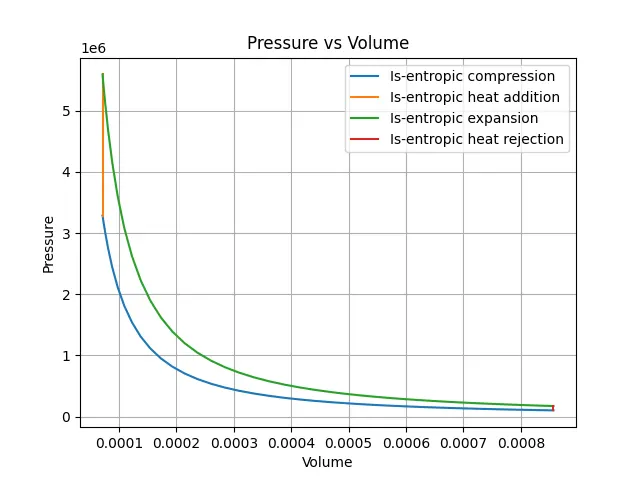
7. For Plotting p-v diagram plt.plot command is used from matplotlib.pyplot module.
8. For the compression stage, the starting and ending crank angles are 180 and 0.
9. for the expansion stage, the starting and ending crank angles are 0 and 180.
10. Let us consider the value to be iterated is 50 accordingly v null set is created to store the value using append command.

Our Code is attached below:

import math

import matplotlib.pyplot as plt

def engine_kinematics(bore, stroke, con_rod, cr, start_angle, end_angle):

    # engine Parameters
    a = stroke / 2
    R = con_rod / a
    v_s = (math.pi / 4) * pow(bore, 2) * stroke
    v_c = v_s / (cr - 1)
    sc = math.radians(start_angle)
    ec = math.radians(end_angle)
    num_values = 50
    dtheta = (ec - sc) / (num_values - 1)
    v = []
    for i in range(0, num_values):
        theta = sc + i * dtheta
        term1 = 0.5 * (cr - 1)
        term2 = R + 1 - math.cos(theta)
        term3 = pow(pow(R, 2) - pow(math.sin(theta), 2),0.5)
        v.append((1 + term1 * (term2 - term3)) * v_c)
    return v

# Input
p1 = 101325
t1 = 500
gamma = 1.4
t3 = 2300

# Geometric parameter
bore = 0.1
stroke = 0.1
con_rod = 0.15
cr = 12

# Volume computation
v_s = (math.pi / 4) * pow(bore, 2) * stroke
v_c = v_s / (cr-1)
v1 = v_s + v_c

# State point 2
v2 = v_c
# p2*v2^gamma = p1*v1^gamma
p2 = p1*pow(v1, gamma)/pow(v2, gamma)
# p2v2/t2 = p1v1/t1 | rhs = p1v1/t1 | lhs = p2v2/t2
rhs = p1 * v1 / t1
t2 = p2 * v2 / rhs

v_compression = engine_kinematics(bore, stroke, con_rod, cr, 180, 0)
constant = p1 * pow(v1, gamma)
p_compression = []
for V in v_compression:
    p_compression.append(constant / pow(V, gamma))

# State point 3
v3 = v2

# p3v3/t3 = p2v2/t2 | rhs = p2v2/t2 | p3 = rhs * t3/v3
rhs = p2 * v2 / t2
p3 = rhs * t3 / v3
v_expansion = engine_kinematics(bore, stroke, con_rod, cr, 0, 180)
constant = p3 * pow(v3, gamma)
p_expansion = []
for V in v_expansion:
    p_expansion.append(constant / pow(V, gamma))

# State point 4
v4 = v1

# p4v4^gamma = p3v3^gamma
p4 = p3 * pow(v3, gamma) / pow(v4, gamma)

# p4v4/t4 = rhs
t4 = p4 * v4 / rhs

# Work done Efficiency
m = 1
cv = 714
Heat_supplied = m*cv*(t3-t2)/1000
Heat_rejected = m*cv*(t4-t1)/1000
Net_work = Heat_supplied - Heat_rejected
W = m*cv*((t3-t2)-(t4-t1))/1000
thermal_efficiency = (1-(1/pow(cr,(gamma-1))))*100
print('Heat Supplyed = ', Heat_supplied, 'Kj/sec')
print('Heat Rejected = ', Heat_rejected, 'Kj/sec')
print('Net Work = ', Net_work, 'Kj/sec')
print('Work Done = ', W, 'Kj/sec')
print('Thermal efficiency is : ', thermal_efficiency, '%')

# Plot
plt.figure()
plt.plot(v_compression, p_compression, label='Is-entropic compression')
plt.plot([v2,v3],[p2,p3], label='Is-entropic heat addition')
plt.plot(v_expansion, p_expansion, label='Is-entropic expansion')
plt.plot([v4,v1], [p4,p1], label='Is-entropic heat rejection')
plt.xlabel('Volume')
plt.ylabel('Pressure')
plt.title('Pressure vs Volume')
plt.legend()
plt.grid('on')
plt.show()

Output Graphs:

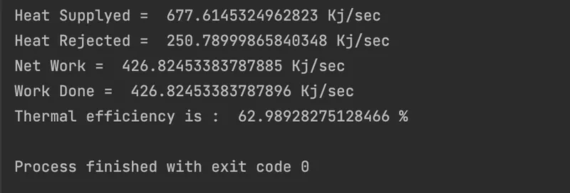
Output Result :

Conclusion :

The Desired p-v diagram of otto cycle is plotted using python programming language using desired array of volume and for different crank angle.