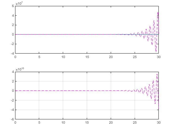
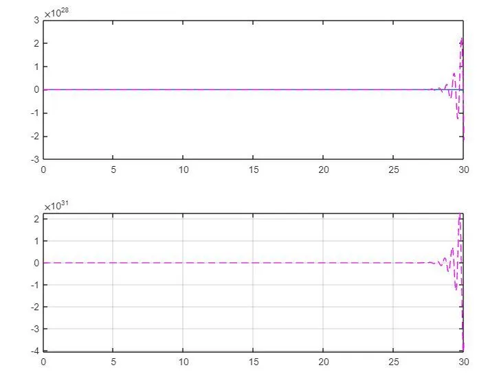
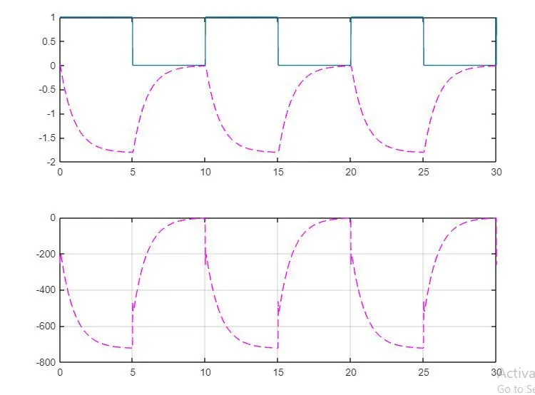
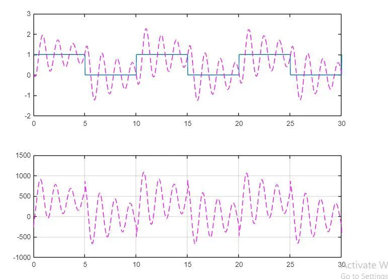
Project: Spring Mass Damper System with PID Controller:
1st of all Differencial equation of Spring Mass Damper System is
m*x_dot_dot + c*x_dot + k*x = f(t)
x_dot_dot = [f(t) - c*x_dot - k*x] / m
state space representation :
x1_dot = x2 = velocity
x_dot_dot = x2_dot = Acceleration
x = x1 = displacement
Now spring mass damper system equation is
x2_dot = -(k/m)*x1 - (c/m)*x2 + (1/m) u..........(1)
General structure of PID controller
u(t) = Kp*e(t) + Ki int[e(t)]dt + kd*e(t)/dt
e(t) = error signal
put error signal (xref-x1) inside the u(t) equation,
u(t) = -Kp*(xref-x1) - Ki * int(xref-x1) + kd*x2
Feedback control law u = -kx
so u = Kp*(xref-x1) + Ki * int(xref-x1) - kd*x2
put u(t) inside equation 1
x2_dot = -(k/m)*x1 - (c/m)*x2 + (1/m) [Kp*(xref-x1) + Ki * int(xref-x1) - kd*x2]
It is the state-space representatioin for te spring mass damping system with PID control design.
% Nominal design Parameters of spring mass system
m = 3.6;
k = 400;
c = 100;
% design Parameters of spring mass system
fn = 1.0;
wn = 2*pi*fn;% wn= 2*pi*fn = sqrt(k/m)
zeta = 0.5; % under dampped system
% Desired Poles
p1= -zeta*wn+wn*sqrt(zeta^2-1);
p2= -zeta*wn-wn*sqrt(zeta^2-1);
P= [p1;p2];
% A and B matirces
A= [0 1;-k/m 0];
B= [0;1/m];
% Pole Placement design
K = place(A,B,P);
% Initial condition
x10 = 0.01;
x20 = 0.0;
% Dynamics
% x_dot = x2
% x2_dot = (k/m)*x1 - (c/m)*x2 + (1/m)*u
% u = [Kp*(x1ref-x1)-Kd*x2+Ki*int(x1ref-x1)*dt] (spring mass damper system with PID Design)
% x2_dot = (k/m)*x1 - (c/m)*x2 + (1/m)*[Kp*(x1ref-x1)-Kd*x2+Ki*int(x1ref-x1)*dt]
% x1ref = pulse generator reference signal with magnitude 1.0 and duration 10.0 seconds
when we run above script
springmassdamperPID
K
K =
-257.8777 22.6195
Kp = -257.8
Kp =
-257.8000
Kd = 22.6
Kd =
22.6000
k/m
ans =
111.1111
c/m
ans =
27.7778
we can change value of Ki and see the behaviour.
Summery:
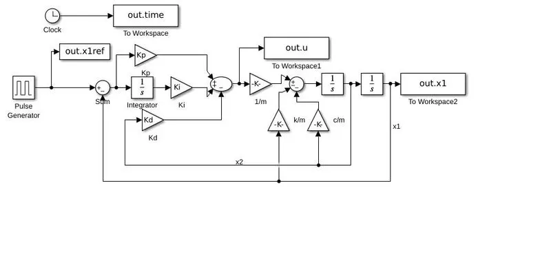
modeling start with pulse generator as given above take as a reference signal with magnitude 1.0 and duration 10.0 seconds. put Kp and Kd value from pole pacement design as we used command place for obtaining K. Here Ki remain changing as per requirement.we used gain block to insert the value of Kp,Ki,Kd,1/m and c/m. then after we used integrator block for velocity and displacement value. sum injection is necessery for subtraction and adition.at the end we check the behaviour of x1 with respect to xref and see the behavior of input force u.
Model:
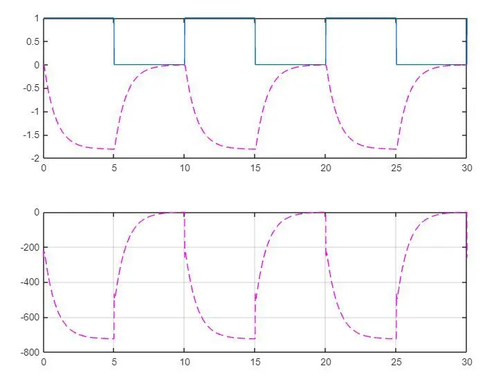
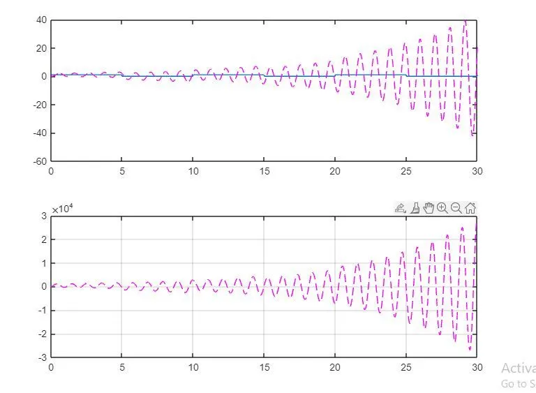
Plotting: Ki = 0.0;
subplot(211);plot(out.time,out.x1ref);grid;hold;
Current plot held
subplot(211);plot(out.time,out.x1,'m--');grid;
subplot(212);plot(out.time,out.u,'m--');grid;
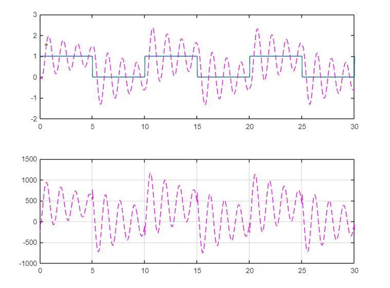
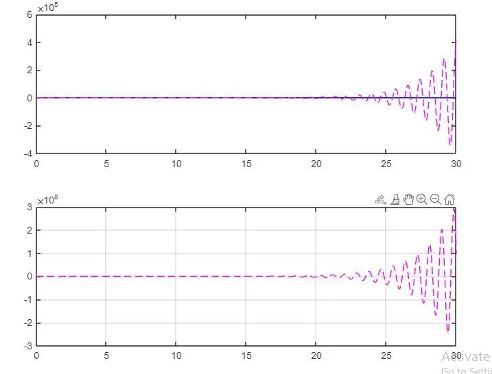
Ki = 2500.0;
subplot(211);plot(out.time,out.x1ref);grid;hold;
Current plot held
subplot(211);plot(out.time,out.x1,'m--');grid;
subplot(212);plot(out.time,out.u,'m--');grid;
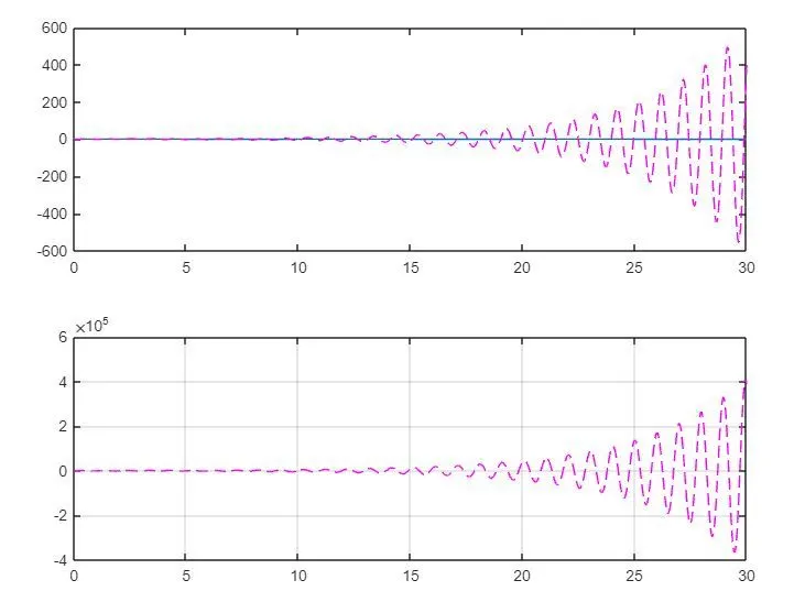
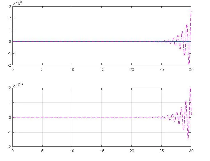
Ki = 5000.0;
subplot(211);plot(out.time,out.x1ref);grid;hold;
Current plot held
subplot(211);plot(out.time,out.x1,'m--');grid;
subplot(212);plot(out.time,out.u,'m--');grid;
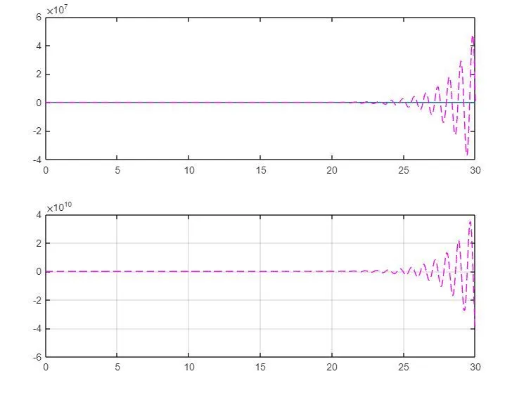
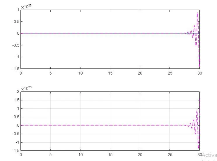
Ki = 7500.0;
subplot(211);plot(out.time,out.x1ref);grid;hold;
Current plot held
subplot(211);plot(out.time,out.x1,'m--');grid;
subplot(212);plot(out.time,out.u,'m--');grid;
Ki = 10000.0;
subplot(211);plot(out.time,out.x1ref);grid;hold;
Current plot held
subplot(211);plot(out.time,out.x1,'m--');grid;
subplot(212);plot(out.time,out.u,'m--');grid;
Ki = 20000.0;
subplot(211);plot(out.time,out.x1ref);grid;hold;
Current plot held
subplot(211);plot(out.time,out.x1,'m--');grid;
subplot(212);plot(out.time,out.u,'m--');grid;
Last we changed the zeta value from 0.5 to 0.9 and check the behaviour as above.
zeta = 0.9;
chage the value of zeta in matlab script 'PID_design.m' and run the file.
Ki = 0.0;
subplot(211);plot(out.time,out.x1ref);grid;hold;
Current plot held
subplot(211);plot(out.time,out.x1,'m--');grid;
subplot(212);plot(out.time,out.u,'m--');grid;
Ki = 2500.0;
subplot(211);plot(out.time,out.x1ref);grid;hold;
Current plot held
subplot(211);plot(out.time,out.x1,'m--');grid;
subplot(212);plot(out.time,out.u,'m--');grid;
Ki = 5000.0;
subplot(211);plot(out.time,out.x1ref);grid;hold;
Current plot held
subplot(211);plot(out.time,out.x1,'m--');grid;
subplot(212);plot(out.time,out.u,'m--');grid;
Ki = 7500.0;
subplot(211);plot(out.time,out.x1ref);grid;hold;
Current plot held
subplot(211);plot(out.time,out.x1,'m--');grid;
subplot(212);plot(out.time,out.u,'m--');grid;
Ki = 10000.0;
subplot(211);plot(out.time,out.x1ref);grid;hold;
Current plot held
subplot(211);plot(out.time,out.x1,'m--');grid;
subplot(212);plot(out.time,out.u,'m--');grid;
Ki = 20000.0;
subplot(211);plot(out.time,out.x1ref);grid;hold;
Current plot held
subplot(211);plot(out.time,out.x1,'m--');grid;
subplot(212);plot(out.time,out.u,'m--');grid;
Conclution: here we can see the both the damping condition where when we increased the value of Ki oscillation behaviour decrease and design crreation gets smoother. overshoot gets less and looks good.