Challenge

Week 2 Air standard Cycle

VVikash Kumar15 Mar 2023

AIM: Write a python program for an Otto Cycle and make plots for it.

Objective:

The objective of the project is to write a python program for an Otto Cycle and make a PV graph of their output result. Also caclulate thier thermal efficiency of the engine.

Concept of Otto Cycle

The Otto cycle is a cycle of engine operation which requires four strokes of the piston: for induction, compression, ignition, and exhaust. The fuel and air mixture is compressed before combustion is started by an electrical spark, in which the combustion of the working fluid-gasoline and air (oxygen), changes the motion in the piston.

PV and TS diagram of an Otto Cycle

For better understanding, these are the following step on the PV diagram of an Otto cycle

Process 1 to 2: Adiabatic Compression
Process 2 to 3: Constant pressure heat addition
Process 3 to 4: Adiabatic Expansion
Process 4 to 1: Constant pressure heat rejection

Basic Equation:

For Adiabatic Process:

`P.(V)^gamma = Constant`

Ideal Gas law:

`(P.V)/T = constant`

Variation of Volume in cylinder with crank angle is given by:

`V/(Vc) = 1 + 1/2*(Cr - 1)[R + 1 - costheta - (R^2 - sin^2theta)^(1/2)]`

Where, `R`= Connecting rod length / Crank pin radius

Crank pin radius = stroke/2

Cr = Compression ratio

`Vc` = Clearance volume

P = pressure

V = volume

T = temperatute

Thermal Efficiency,

`ita (%) = [1 - (1/(cr^(gamma - 1)))]* 100` (in percent)

PROCEDURE AND EXPLAINATION FOR PYTHON

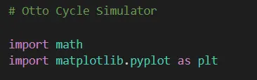
Step-1: Before writing the program first we have to import command to import libraries which will be used in mathematical operation and plotting.

Step-2: Basic Program
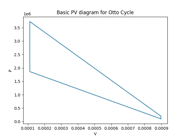
First, we are going to do the basic program with the help of defined state variable points.

Basic_Code

# Otto Cycle Simulator

import math

import matplotlib.pyplot as plt

# pressure (pa) & Temp (K)

p1 = 101325

t1 = 500

# geometric parameter

bore = 0.1

stroke = 0.1

con_rod = 0.15

cr = 8

gamma = 1.4

t3 = 2300

# volume computation (swept volume and clearance volume)

v_s = math.pi/4*pow(bore,2)*stroke

v_c = v_s/(cr-1)

v1 = v_c + v_s

# state point 2

v2 = v_c

# Pressure p2.v2^gamma = p1.v1^gamma

p2 = p1*pow(v1,gamma)/pow(v2,gamma)

# p2v2/t2 = p1v1/t1 | p1v1/t1 = rhs | t2 = p2v2/rhs

rhs = p1*v1/t1

t2 = p2*v2/rhs

# state point 3

v3 = v2

# p2v3/t3 = p2v2/t2 | p2v2/t2 = rhs

rhs = p2*v2/t2

p3 = rhs*t3/v3

# state point 4

v4 = v1

# p4v4^gamma = p3v3^gamma

p4 = p3*pow(v3,gamma)/pow(v4,gamma)

# p4v4/t4 = p3v3/t3 | p3v3/t3 = rhs

rhs = p3*v3/t3

t4 = rhs*p4/v4

# plotting Otto cycle graph

plt.plot([v1,v2,v3,v4,v1],[p1,p2,p3,p4,p1])

plt.title('Basic PV diagram for Otto Cycle')

plt.xlabel('V')

plt.ylabel('P')

plt.savefig('Basic PV diagram for Otto Cycle')

plt.show()

Result of basic program

From the above plot, we can see that the compression and Expansion processes are shown linear, which is practically not possible. Hence to make the proper plot we need the Engine kinematics equation as discussed below.

Step-3: Defining Engine Kinematics function

To plot correctly, we need the following two things.

Thermodynamic relation during compression and Expansion.
Piston kinematics to determine How the volume change from TDC to BDC and how combustion volume changes as a function of the crank angle.

Here, we are taking all the parameters the same as discussed in step 1 and 2, but we need a different formula for the calculation of the volume change inside the combustion chamber. The required relationship we can get by the following formula. The Formula for the Engine kinematics is as follows.

`V/(Vc) = 1 + 1/2*(Cr - 1)[R + 1 - costheta - (R^2 - sin^2theta)^(1/2)]`

To use this formula in the program we simplified it. Hence, To simplify the formula we divided formula into three sub formulas (terms) as follows.

`term1 = 0.5 * (cr - 1)`

`term2 = 1 + R - costheta`

`term3 = (R^2 - sin^2theta)^(1/2)`

At last, After combining the terms to get the final formula,

`V = (1 + term1*(term2 - term3))*Vc`

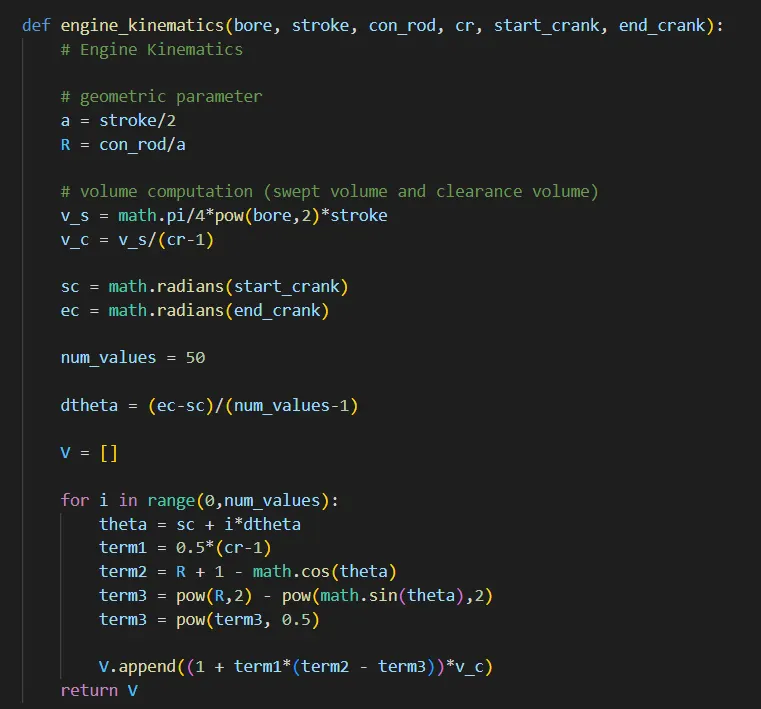
After that our Engine kinematics formula is used as a function in the program is as shown below.

Where:

We need the formula of engine kinematics to create the volume Arrays concerning the compression and Expansion Processes. After that, we can use it in our Otto cycle Program. Also, we need to calculate the pressure that corresponds to the volume. Therefore, We defined the Engine kinematics as the function.
Since we have a function so we need not pre-define the value of the parameters related to it such as values of bore, stroke, connecting rod length, etc.
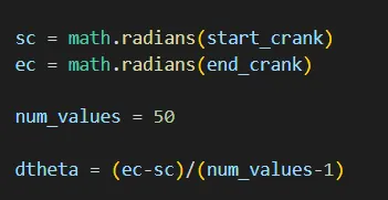
Now defining the sc and ec (i.e starting crank angle and ending crank angle). Because we want to get several values between the starting crank and ending crank position and each of those values we need to get the volume. hence using ec and sc and assigning it to the dtheta which is known as a crank angle spacing. Also defined the number of values is equal to 50 as follows.

Now we can form a crank angle array. to do that we are using for-loop. For loop use to repeat the set of actions multiple times. The empty volume array indicates that when for loop executed each time the value calculated in the for-loop gets store in the empty array.
But to generate the multiple values we need one more command called as append.".append" is used to continuously append (increase) the value and store it in the empty array.
using "return V" to get multiple output values of volume.

Step-4: Defining the Compression and Expansion processes

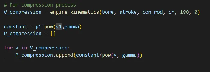
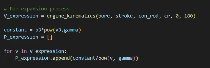
To define the compression and Expansion processes in the program we took help to the engine kinematic function as shown below.

State point 2 (Compression process)

State point 3 (expansion process)

Where:

For loop is used to get multiple values of the volume and pressure and store it in the empty array using Append command.

For compression, the taken starting crank angle is at 180 degrees and the ending crank angle is 0 degree (i.e piston moves from BDC to TDC). Similarly, For Expansion, the taken starting crank angle is at 0 degrees and the ending crank angle is 180 degrees (i.e piston moves from TDC to BDC).

Note: Here We took the crank angle for reference to the compression and expansion process not a movement of the piston. Also, suction and exhaust are neglected.

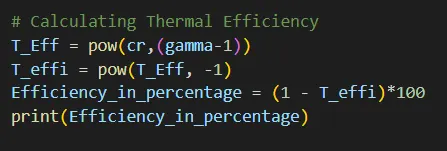
Step-5: Calculating Thermal Efficiency

We are using the efficiency formula for the ideal otto cycle in percentage so that we can determine the efficiency of the otto cycle. The Thermal efficiency formula in percentage is as following.

`ita (%) = [1 - (1/(cr^(gamma - 1)))]* 100`

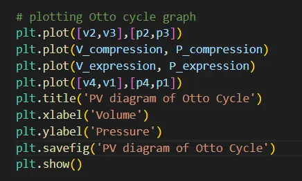
Step-6: Creating Plot

After defining all the terms we need the output so to do that we are using the plot command and plotted all the processes.

After properly arranging the program we get out the desired program and output which is shown below.

Python Program (Final):

# Otto Cycle Simulator

import math

import matplotlib.pyplot as plt

def engine_kinematics(bore, stroke, con_rod, cr, start_crank, end_crank):

# Engine Kinematics

# geometric parameter

a = stroke/2

R = con_rod/a

# volume computation (swept volume and clearance volume)

v_s = math.pi/4*pow(bore,2)*stroke

v_c = v_s/(cr-1)

sc = math.radians(start_crank)

ec = math.radians(end_crank)

num_values = 50

dtheta = (ec-sc)/(num_values-1)

V = []

for i in range(0,num_values):

theta = sc + i*dtheta

term1 = 0.5*(cr-1)

term2 = R + 1 - math.cos(theta)

term3 = pow(R,2) - pow(math.sin(theta),2)

term3 = pow(term3, 0.5)

V.append((1 + term1*(term2 - term3))*v_c)

return V

# pressure (pa) & Temp (K)

p1 = 101325

t1 = 500

# geometric parameter

bore = 0.1

stroke = 0.1

con_rod = 0.15

cr = 8

gamma = 1.4

t3 = 2300

# volume computation (swept volume and clearance volume)

v_s = math.pi/4*pow(bore,2)*stroke

v_c = v_s/(cr-1)

v1 = v_c + v_s

# state point 2

v2 = v_c

# Pressure p2.v2^gamma = p1.v1^gamma

p2 = p1*pow(v1,gamma)/pow(v2,gamma)

# p2v2/t2 = p1v1/t1 | p1v1/t1 = rhs | t2 = p2v2/rhs

rhs = p1*v1/t1

t2 = p2*v2/rhs

# For compression process

V_compression = engine_kinematics(bore, stroke, con_rod, cr, 180, 0)

constant = p1*pow(v1,gamma)

P_compression = []

for v in V_compression:

P_compression.append(constant/pow(v, gamma))

# state point 3

v3 = v2

# p2v3/t3 = p2v2/t2 | p2v2/t2 = rhs

rhs = p2*v2/t2

p3 = rhs*t3/v3

# For expansion process

V_expression = engine_kinematics(bore, stroke, con_rod, cr, 0, 180)

constant = p3*pow(v3,gamma)

P_expression = []

for v in V_expression:

P_expression.append(constant/pow(v, gamma))

# state point 4

v4 = v1

# p4v4^gamma = p3v3^gamma

p4 = p3*pow(v3,gamma)/pow(v4,gamma)

# p4v4/t4 = p3v3/t3 | p3v3/t3 = rhs

rhs = p3*v3/t3

t4 = rhs*p4/v4

# Calculating Thermal Efficiency

T_Eff = pow(cr,(gamma-1))

T_effi = pow(T_Eff, -1)

Efficiency_in_percentage = (1 - T_effi)*100

print(Efficiency_in_percentage)

# plotting Otto cycle graph

plt.plot([v2,v3],[p2,p3])

plt.plot(V_compression, P_compression)

plt.plot(V_expression, P_expression)

plt.plot([v4,v1],[p4,p1])

plt.title('PV diagram of Otto Cycle')

plt.xlabel('Volume')

plt.ylabel('Pressure')

plt.savefig('PV diagram of Otto Cycle')

plt.show()

OUTPUT RESULT:

By Executing the Program we get our required output as,

Otto cycle plot of PV diagram and
Thermal efficiency in percentage.

1. PV Diagram

Compression ratio = 8

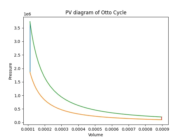
Now we can see that the compression and expansion process in the above figure is a curve, which is practically possible but in previous PV graph it shown linear which is not acceptable but now in the above figure adiabatic process is a curve.

2. Thermal Efficiency ( in percentage)

Thermal Efficincy = `56.47%`

CONCLUSION

We create a program for Air Standard Cycle (Otto Cycle) with the help of Python. And plot the output result of PV diagram, also demonstrate thermal efficiency of otto cycle.

Week 2 Air standard Cycle

Ship work like this
in your own course.

Talk to a career counsellor

Ship work like thisin your own course.

Talk to a career counsellor

Ship work like this
in your own course.