Week 2 Air standard Cycle

AIM :

Based on the concepts you have learned during the forward kinematics routine, write code that can solve an otto cycle and make plots for it.

OBJECTIVE :

1. Your code should create a PV diagram

2. You should output the thermal efficiency of the engine.

THEORY

thermal efficiency of OTTO CYCLE

In general, the thermal efficiency, η_th, of any heat engine is defined as the ratio of the work it does, W, to the heat input at the high temperature, Q_H.

The heat absorbed occurs roughly at a constant volume during the combustion of the fuel-air mixture, when the spark occurs. Since during an isochoric process, there is no work done by or on the system, the first law of thermodynamics dictates ∆U = ∆Q. Therefore, the heat added and rejected is given by:

Q_add = mc_v (T₃ – T₂)

Q_out = mc_v (T₄ – T₁)

Substituting these expressions for the heat added and rejected in the expression for thermal efficiency yields:

We can simplify the above expression using the fact that the processes 1 → 2 and from 3 → 4 are adiabatic, and for an adiabatic process, the following p,V,T formula is valid:

It can be derived that:

THE CODE :

import math
import matplotlib.pyplot as plt


def engine_kinematics(bore,stroke,con_rod,Cr,theta_begin,theta_end):
	
	a = stroke/2
	R = stroke/a

	N_theta = 50
	
	SC = math.radians(theta_begin)
	EC = math.radians(theta_end)
	dtheta = ( EC - SC )/ (N_theta-1)
	V = []

	for i in range(0,N_theta):
		theta = EC + i*dtheta
		term1= 0.5*(Cr-1)
		term2 = R+1-math.cos(theta)
		term3 = pow(R,2)-pow(math.sin(theta),2)
		term3 = pow(term3,0.5)
		V.append((1+term1*(term2-term3))*V_c)
	return V	

#inputs
p1 = 10500
t1 = 500
gamma = 1.4
t3 = 2500
#gerometric parameter
bore = 0.1
stroke = 0.1
con_rod = 0.2
Cr = 12

#state point 1
V_s = (math.pi/4)*pow(bore,2)*stroke
V_c = V_s/(Cr-1)
V1 = V_s+V_c
#Sate vale 2
V2 = V_c

#P1 * V1^gamma = P2 * V2^gamma gas equation
p2 = p1*pow(V1,gamma)/pow(V2,gamma)

#P1*V1/T1 = P2*V2/T2 = rhs
rhs=p1*V1/t1
t2 = p2*V2/rhs
V_compression = engine_kinematics(bore,stroke,con_rod,Cr,180,0)
const = p1*pow(V1,gamma)
p_compression=[]

for v in V_compression:
	p_compression.append(const/pow(v,gamma))

#state value 3

V3 = V2
p3 = rhs*t3/V3

#State pont 4

V_expansion = engine_kinematics(bore,stroke,con_rod,Cr,0,180)
const = p3*pow(V3,gamma)
p_expansion=[]

for v in V_expansion:
	p_expansion.append(const/pow(v,gamma))


V4 = V1
#P1 * V1^gamma = P2 * V2^gamma gas equation
p4 = p3*pow(V3,gamma)/pow(V4,gamma)

t4 = p4*V4/rhs

Eff=1-(t1/t2)
print(Eff)

plt.plot([V2,V3],[p2,p3])
plt.plot(V_compression,p_compression)
plt.plot(V_expansion,p_expansion)
plt.plot([V4,V1],[p4,p1])
plt.show()

Explanation

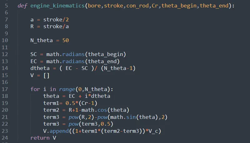
First of all, we declare a function for the volume from governing equation as given below and loop the theta quantity to get different volume over the theta variant.

Now we call for all the inputs required to plot a PV diagram as below.

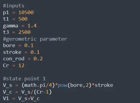
Volume for the first state point is calculated from swept volume and clearance volume.

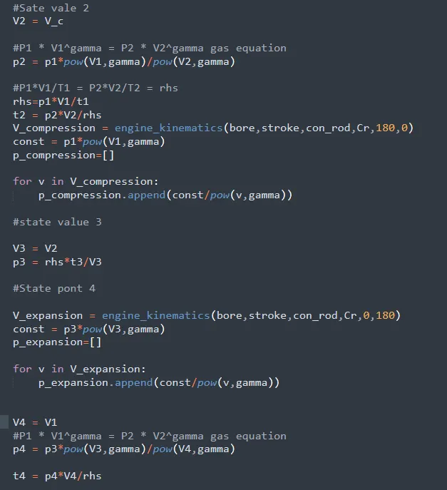
then we equate state point values for 2,3,4 using the gas laws ie Boyles and ideal gas equation.

for compression and expansion volume, we call the function with appropriate theta angles. Then we declare an empty array of pressure. then use PV relation to find pressure corresponding to these volumes and append the command to save all the values inside the empty array.

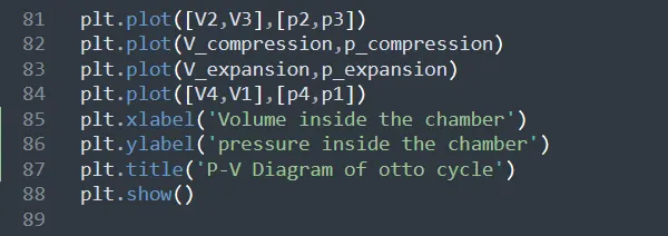
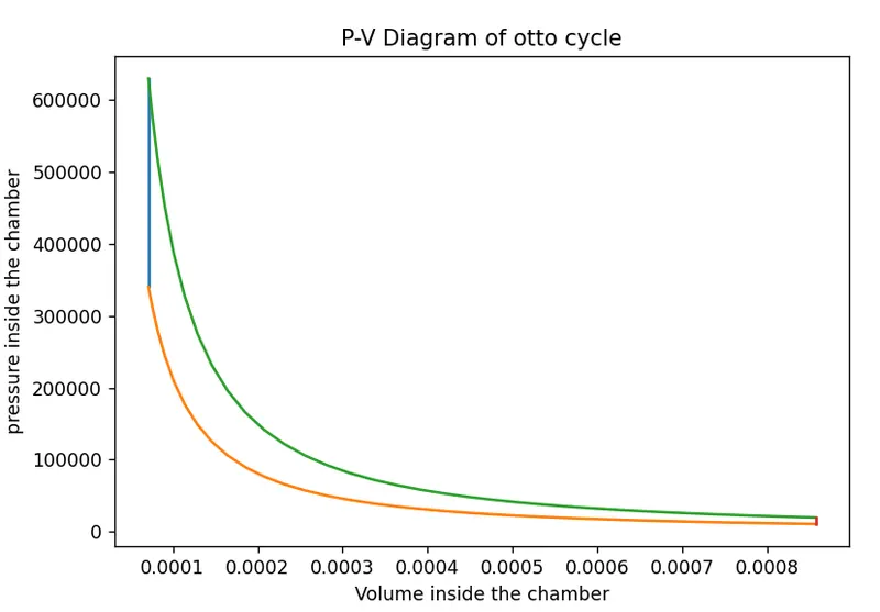
Using pltplot command we plot the PV diagram using all the inputs that we calculated.

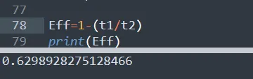
Now we have to calculate the thermal efficiency for which we use the equation 1-(t1/t2) as given below.

RESULTS.

Thermal efficiency = 1-(t1/t2) = 0.6298928275128466

CONCLUSION

The desired p-v diagram of the otto cycle is plotted using python programming language by using an array of volumes and different crank angles.