Week 2 Air standard Cycle
otto cycle
An Otto cycle is an idealized thermodynamic cycle that describes the functioning of a typical spark ignition piston engine. It is the thermodynamic cycle most commonly found in automobile engines.
"""
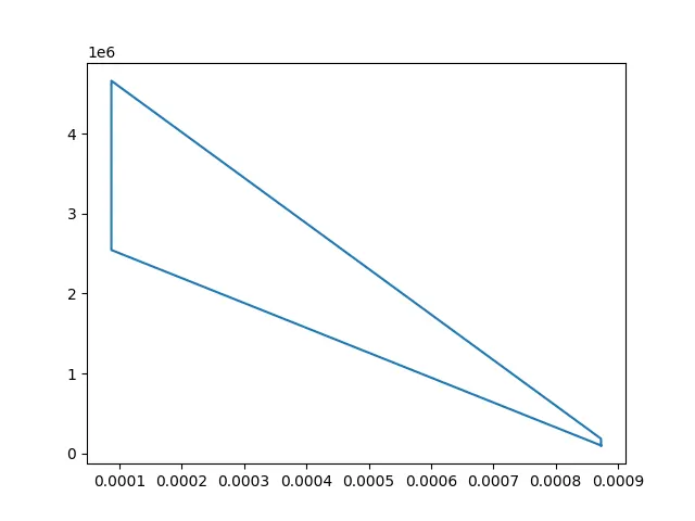
Otto cycle Pressure and Volume
"""
import math
import matplotlib.pyplot as plt
# Input
P1 = 101325
t1 = 500
gamma = 1.4
t3 = 2300
# geomatical parameters
bore = 0.1
stroke = 0.1
con_rod = 0.15
cr = 10
# volume computation
V_s = (math.pi/4)* pow(bore,2)*stroke
V_c = V_s/(cr-1)
V1 = V_c + V_s
# start point 2
V2 = V_c
# P2 V2 ^ gama =P1 V1 ^ gama
P2 =P1*pow(V1,gamma)/pow(V2,gamma)
#P2 v2 /t2 = P1 V1 /t1
#rhs =P1 V1 /t1 |P2V2 /t2 = rhs/ t2 = P2 V2 /rhs
RHS = P1 * V1 /t1
t2 = P2* V2 /RHS
# state point 3
V3 = V2
# P3V3 /t3 = P2 * V2 /t2 | rhs = P2 V2 /t2 | P3 = rhs*t3/V3
RHS = P2 * V2/t2
P3 = RHS*t3/V3
# state point 4
V4 = V1
# P4 V4 ^gamma = P3 V3 ^gamma
P4 = P3 *pow(V3,gamma)/pow (V4,gamma)
# P4 V4/t4 = RHSC
t4 = P4 * V4/RHS
plt.plot([V1,V2,V3,V4,V1],[P1,P2,P3,P4,P1])
plt.show()
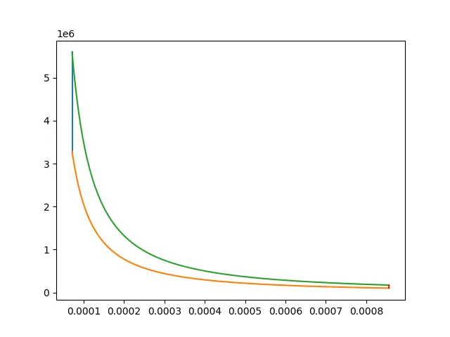
Function definition for kinematics
import math
bore = 0.10
stroke = 0.1
con_rod = 0.15
cr = 12
a = stroke/2
R = con_rod/a
theta = math.radians(0)
V_S = math.pi*(1/4)*pow(bore,2)*stroke
V_C = V_S/(cr-1)engine kinematics
term1 = 0.5*(cr-1)
term2 = R+1 -math.cos(theta)
term3 = pow(R,2)-pow(math.sin(theta),2)
term3 = pow(term3,0.5)
V = (1+term1*(term2-term3))*V_C
"""
Otto cycle creation for engine kinematics
"""
import math
import matplotlib.pyplot as plt
"""
engine kinematics
"""
def engine_kinematics(bore,stroke,con_rod,cr,strat_crank,end_crank):
a = stroke/2
R = con_rod/a
num_value = 100
sc = math.radians(strat_crank)
ec = math.radians(end_crank)
dtheta = (sc-ec)/(num_value-1)
V_S = math.pi*(1/4)*pow(bore,2)*stroke
V_C = V_S/(cr-1)
V =[]
for i in range(0,num_value):
theta = sc+ i*(dtheta)
V_S = math.pi*(1/4)*pow(bore,2)*stroke
V_C = V_S/(cr-1)
term1 = 0.5*(cr-1)
term2 = R+1 -math.cos(theta)
term3 = pow(R,2)-pow(math.sin(theta),2)
term3 = pow(term3,0.5)
V.append((1+term1*(term2-term3))*V_C)
return V
# Input
P1 = 101325
t1 = 500
gamma = 1.4
t3 = 2300
# geomatical parameters
bore = 0.1
stroke = 0.1
con_rod = 0.15
cr = 12
# volume computation
V_s = (math.pi/4)* pow(bore,2)*stroke
V_c = V_s/(cr-1)
V1 = V_c + V_s
# start point 2
V2 = V_c
# P2 V2 ^ gama =P1 V1 ^ gama
P2 =P1*pow(V1,gamma)/pow(V2,gamma)
#P2 v2 /t2 = P1 V1 /t1
#rhs =P1 V1 /t1 |P2V2 /t2 = rhs/ t2 = P2 V2 /rhs
RHS = P1 * V1 /t1
t2 = P2* V2 /RHS
V_compression= engine_kinematics(bore,stroke,con_rod,cr,180,0)
constant = P1*pow(V1,gamma)
P_compression = []
for v in V_compression:
P_compression.append(constant/pow(v,gamma))
# state point 3
V3 = V2
# P3V3 /t3 = P2 * V2 /t2 | rhs = P2 V2 /t2 | P3 = rhs*t3/V3
RHS = P2 * V2/t2
P3 = RHS*t3/V3
V_expansion= engine_kinematics(bore,stroke,con_rod,cr,0,180)
constant = P3*pow(V3,gamma)
P_expansion = []
for v in V_expansion:
P_expansion .append(constant/pow(v,gamma))
# state point 4
V4 = V1
# P4 V4 ^gamma = P3 V3 ^gamma
P4 = P3 *pow(V3,gamma)/pow(V4,gamma)
# P4 V4/t4 = RHS
t4 = P4 * V4/RHS
plt.plot([V2,V3],[P2,P3])
plt.plot(V_compression,P_compression)
plt.plot(V_expansion,P_expansion)
plt.plot([V4,V1],[P4,P1])
plt.show()
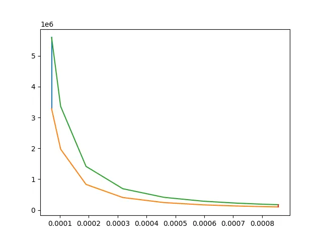
number of iteration 10
number of iteration 100