Week 2 Air standard Cycle

Air standard Cycle

Aim: Write a code that can solve an otto cycle and plot of it

Objectives:

• To write a basic code to solve the Air standard cycle.
• To find out the efficiency of the Air standard cycle and with trial and error method optimize engine efficiency.
• To plot the results obtained to visualize the actual scenario.

Introduction:

An Otto cycle is an idealized thermodynamic cycle that describes the functioning of a typical spark ignition piston engine

Processes:

1. Process 0–1 a mass of air is drawn into a piston/cylinder arrangement at constant pressure.
2. Process 1–2 is an isentropic compression of the charge as the piston moves from the bottom dead center (BDC) to the top dead center (TDC).
3. Processes 2–3 is a constant-volume heat transfer to the working gas from an external source while the piston is at top dead center. This process is intended to represent the ignition of the fuel-air mixture and the subsequent rapid burning.
4. Process 3–4 is an isentropic expansion.
5. Process 4–1 completes the cycle by a constant-volume process in which heat is rejected from the air while the piston is at the bottom dead center.
6. Process 1–0 the mass of air is exhausted to the atmosphere in a constant pressure process.

Required formulas:

Swept volume:

Vs = n*(pi/4)*(bore)^2*stroke

where,

n= no of cylinder

Vc= cylinder swept volume [cm3 (cc)]

BDC = Bottom Dead Center TDC = Top Dead Center

Clearance volume:

Vc= Vs/(Cr-1)

V1 = Vs+ Vc

V2 = Vc

where,

Cr=compression ratio

Compression ratio:

Cr=(Vs+ Vc)/ Vc

Isentropic proccess:

P*V^γ= constant

Ideal gas equation:

PV=mRT

Efficiency:

η=(Cr-1)/Cr

Steps/logic:

• Define inputs such as starting temperature, atmospheric pressure, gamma, and combustion temperature.
• Calculate the pressure at compression stroke which is an isentropic process with the equation PV^gamma = constant.
• And calculate the unknown temperature using the ideal gas equation PV=mRT.
• For compression and expansion phases we have the formula to calculate volume at compression and expansion. create a function to calculate values.
• Call a function and calculate the values of pressure at compression and pressure at expansion.
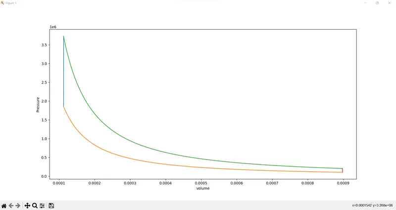
• After getting all the values using the plot command we should plot all four phases.
• At last, calculate the efficiency of the processes using the formula = 1 - (t2/t1)

source code:

"""
Otto cycle simulator vinod
"""

import math
import matplotlib.pyplot as plt

def engine_kinematics(bore,stroke,con_rod,cr,start_crank,end_crank):

    """
    """
    #geometric parameters
    a = stroke/2
    R = con_rod/a

    #volume parameters
    v_s = math.pi*(1/4)*pow(bore,2)*stroke
    v_c = v_s/(cr-1)

    sc = math.radians(start_crank)
    ec = math.radians(end_crank)
    num_values = 100
    dtheta = (ec-sc)/(num_values-1)
    v = []

    for i in range(0,num_values):
        theta = sc+i*dtheta
        term1 = 0.5*(cr-1)
        term2 = R+1-math.cos(theta)
        term3 = pow(R,2)-pow(math.sin(theta),2)
        term3 = pow(term3,0.5)

        v.append((1+term1*(term2-term3))*v_c)
        
    return v

#inputs
p1 = 101325
t1 = 600
gamma = 1.4
t3 = 2100

#geometric parameters
bore = 0.3
stroke = 0.2
con_rod = 0.15
cr = 10

#volume computation
v_s = (math.pi/4)*pow(bore,2)*stroke
v_c = v_s/(cr-1)
v1 = v_c+v_s

#state point 2 
v2 = v_c

#p2v2^gamma = p1v1^gamma
p2 = p1*pow(v1,gamma)/pow(v2,gamma)

#p2v2/t2 = p1v1/t1 | rhs = p1v1/t1 | p2v2/t2 = rhs | t2 = p2v2/rhs
rhs = p1*v1/t1 
t2 = p2*v2/rhs
V_compression = engine_kinematics(bore,stroke,con_rod,cr,180,0)

constant = p1*pow(v1,gamma)

p_compression = []

for v in V_compression:
    p_compression.append(constant/pow(v,gamma))

#print(p_compression)

#state point 3
v3 = v2

#p3v3/t3 = p2v2/t2 | rhs = p2v2/t2 | p3 = rhs*t3/v3
rhs = p2*v2/t2
p3 = rhs*t3/v3

V_expansion = engine_kinematics(bore,stroke,con_rod,cr,0,180)

constant = p3*pow(v3,gamma)

p_expansion = []

for v in V_expansion:
    p_expansion.append(constant/pow(v,gamma))

#print(p_compression)

#state point 4
v4 = v1

#p4v4^gamma = p3v3^gamma
p4 = p3*pow(v3,gamma)/pow(v4,gamma)

#p4v4/t4 = rhs
t4 = p4*v4/rhs

plt.plot([v2,v3],[p2,p3])
plt.plot(V_compression, p_compression)
plt.plot(V_expansion, p_expansion)
plt.plot([v4,v1],[p4,p1])
plt.xlabel('volume')
plt.ylabel('Pressure')
plt.show()

RESULTS

conclusion:

The Python Code for plotting the P_V diagram of an otto cycle was performed.