Gas power Cycle-Otto Cycle

OBJECTIVE:

To write a code in python that can solve the gas power cycle-Otto cycle, plot the pressure-volume graph and also calculate the thermal efficiency of the cycle.

PROBLEM STATEMENT/THEORY:

We know that on this cycle; petrol, gas and many types of oil engines work. It is the standard of comparison for internal combustion engine. To calulate the thermal efficiency of the otty cycle we need to understand the following processes-

• The point 1 represents that cylinder is full of air with volume V1, pressure p1 and absolute
  temperature T1.
• Line 1-2 represents the adiabatic compression of air due to which p1, V1 and T1 change to
  p2, V2 and T2, respectively.
• Line 2-3 shows the supply of heat to the air at constant volume so that p2 and T2 change to
  p3 and T3 (V3 being the same as V2).
• Line 3-4 represents the adiabatic expansion of the air. During expansion p3, V3 and T3
  change to a final value of p4, V4 or V1 and T4, respectively.
• Line 4-1 shows the rejection of heat by air at constant volume till original state (point 1)
  reaches.

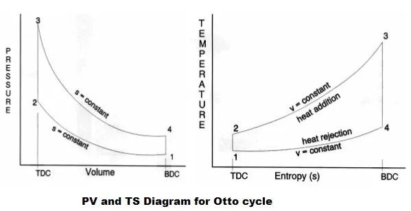
NOTE:(We only plot & study the process for pv graph and not ts)

• Considering 1 kg of air :
  
  Heat supplied at constant volume = cv(T3 – T2).
  Heat rejected at constant volume = cv (T4 – T1).
  However, Work done = Heat supplied – Heat rejected
  W= cv (T3 – T2) – cv (T4 – T1)
  Therefore, Efficiency = Work done/Heat supplied
  
  Efficiency is given by (nu)=`ν`
  =(cv(T3-T2)-cv(T3-T2))/cv(T3-T2)
  =1-((T4-T1)/(T3-T2))

Let compression ratio(cr)=V1/V2

and expansion ratio(er)=V3/V4

(These above mentioned ratios are same for this cycle)

Because, T2/T1=((V1/V2)^γ-1)

so, T2=T1*(cr)^γ-1

Similarly, T3=T4*(cr)^γ-1

Now, inserting these values for T2 and T3 in Efficiency eq. we get,

nu(otto)=1-((1/cr^(γ-1))

This expression is known as the air standard efficiency of the Otto cycle.

It is clear from the above expression that efficiency increases with the increase in the value
of cr, which means we can have maximum efficiency by increasing cr to a considerable extent, but
due to practical difficulties its value is limited to about 8.

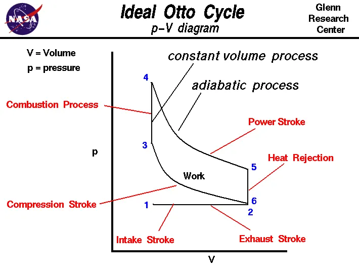
Now, following are the other governing equations required to write the python code-

• Compression ratio(cr)=1+Vs/Vc
• Swept volume(Vs)=π/4(d^2)*L where d=bore diameter and L is the stroke length.
• Clearance volume(Vc)=Vs/(cr-1)
• PV=nRT ----ideal gas eq.
• PV^γ=constant ----adiabatic process eq.

PROCEDURE:

• We first import matplotlib and math libraries.
• Then define a function for engine kinematics in a seperate terminal with bore, stroke, connecting rod, start and end crank angle as predefined.
• Using the formulas and governing equations we append and return the value for V.
• Then back to original tab we copy paste this code and start with the state point 1, where
  p1=101325pa
  t1=323k
• Then we write the code for Vs and Vc(swept and clearance volume) as shown.
• Taking γ=1.4, t3=2000k we compute the Volume.
• Now, in state point 2 we know that v2=Vc, we enter Vc and copy paste the engine kinematics headline (which will run the entire code that we entered in seperate window and compute the values) and enter start and end crank angle as 0 and 180.
• Then, for V_expansion we copy same engine kinematics code and enter crank start and end angle as 180 and 0, then we define an empty array for P_compression and append it as shown.
• For state point 3, we know that v3=v2, we then write the code for p3 and define an empty array for P_expansion and append it as shown.
• Finally for state point 4, we know that v4=v1 and enter the formula for p4.
• Lastly we enter the formula for thermal efficiency and give the print command.
• Also, in the end to plot the graph we give the commands as shown in the code which includes color, linewidth, labels, limits, titles and a grid.

OUTPUT:

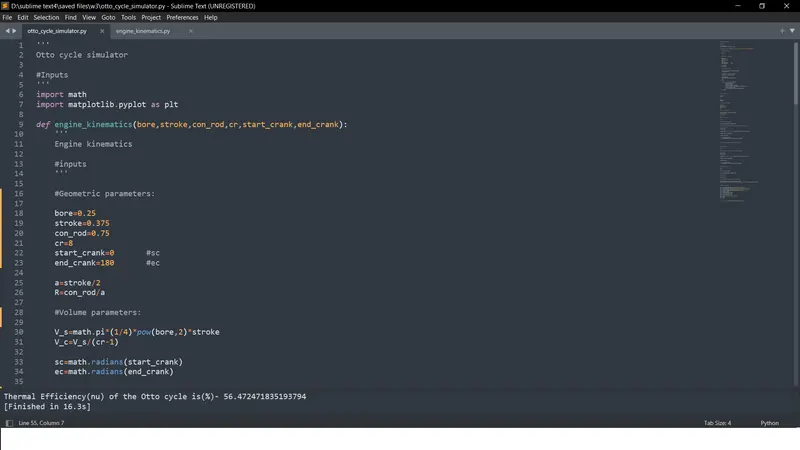
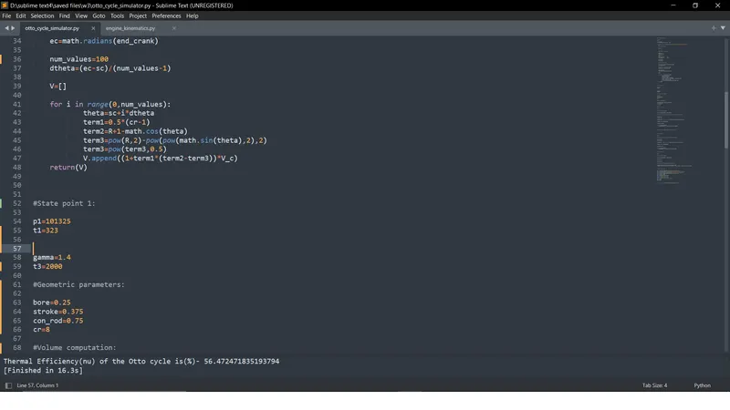
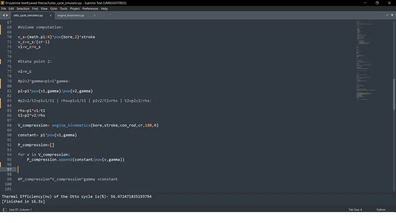
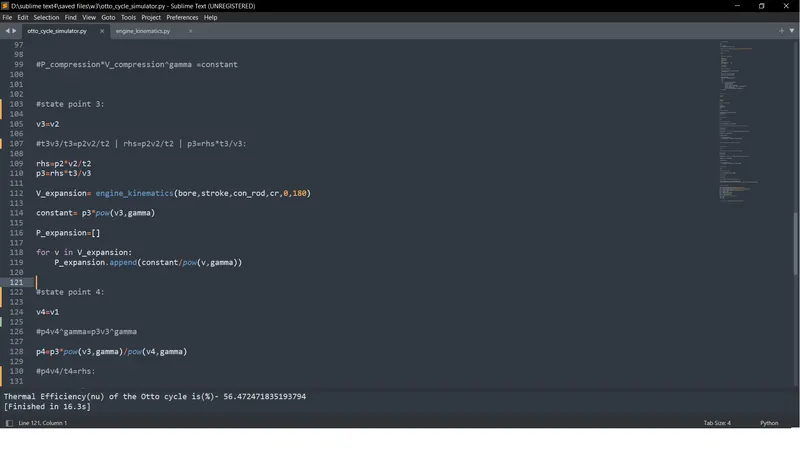
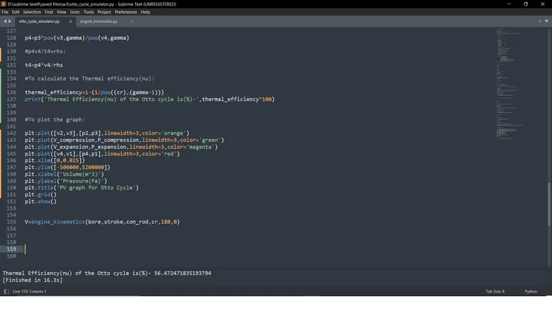
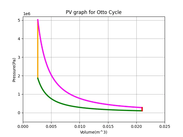
PYTHON CODE:

'''
Otto cycle simulator 
By Prithvi 

#Inputs
'''
import math
import matplotlib.pyplot as plt

def engine_kinematics(bore,stroke,con_rod,cr,start_crank,end_crank):
	'''
	Engine kinematics

	#inputs
	'''

	#Geometric parameters:

	bore=0.25
	stroke=0.375
	con_rod=0.75
	cr=8
	start_crank=0       #sc
	end_crank=180       #ec

	a=stroke/2
	R=con_rod/a

	#Volume parameters:

	V_s=math.pi*(1/4)*pow(bore,2)*stroke
	V_c=V_s/(cr-1)

	sc=math.radians(start_crank)
	ec=math.radians(end_crank)

	num_values=100
	dtheta=(ec-sc)/(num_values-1)

	V=[]

	for i in range(0,num_values):
			theta=sc+i*dtheta
			term1=0.5*(cr-1)
			term2=R+1-math.cos(theta)
			term3=pow(R,2)-pow(pow(math.sin(theta),2),2)
			term3=pow(term3,0.5)
			V.append((1+term1*(term2-term3))*V_c)
	return(V)



#State point 1: 

p1=101325
t1=323


gamma=1.4
t3=2000

#Geometric parameters:

bore=0.25
stroke=0.375
con_rod=0.75
cr=8

#Volume computation:

v_s=(math.pi/4)*pow(bore,2)*stroke
v_c=v_s/(cr-1)
v1=v_c+v_s


#State point 2:

v2=v_c

#p2v2^gamma=p1v1^gamma:

p2=p1*pow(v1,gamma)/pow(v2,gamma)

#p2v2/t2=p1v1/t1 | rhs=p1v1/t1 | p2v2/t2=rhs | t2=p2v2/rhs:

rhs=p1*v1/t1
t2=p2*v2/rhs

V_compression= engine_kinematics(bore,stroke,con_rod,cr,180,0)

constant= p1*pow(v1,gamma)

P_compression=[]

for v in V_compression:
	P_compression.append(constant/pow(v,gamma))



#P_compression*V_compression^gamma =constant



#state point 3:

v3=v2

#t3v3/t3=p2v2/t2 | rhs=p2v2/t2 | p3=rhs*t3/v3:

rhs=p2*v2/t2
p3=rhs*t3/v3

V_expansion= engine_kinematics(bore,stroke,con_rod,cr,0,180)

constant= p3*pow(v3,gamma)

P_expansion=[]

for v in V_expansion:
	P_expansion.append(constant/pow(v,gamma))


#state point 4:

v4=v1

#p4v4^gamma=p3v3^gamma

p4=p3*pow(v3,gamma)/pow(v4,gamma)

#p4v4/t4=rhs:

t4=p4*v4/rhs

#To calculate the Thermal efficiency(nu):

thermal_efficiency=1-(1/pow((cr),(gamma-1)))
print('Thermal Efficiency(nu) of the Otto cycle is(%)=',thermal_efficiency*100)


#To plot the graph:

plt.plot([v2,v3],[p2,p3],linewidth=3,color='orange')
plt.plot(V_compression,P_compression,linewidth=3,color='green')
plt.plot(V_expansion,P_expansion,linewidth=3,color='magenta')
plt.plot([v4,v1],[p4,p1],linewidth=3,color='red')
plt.xlim([0,0.025])
plt.ylim([-500000,5200000])
plt.xlabel('Volume(m^3)')
plt.ylabel('Pressure(Pa)')
plt.title('PV graph for Otto Cycle')
plt.grid()
plt.show()


V=engine_kinematics(bore,stroke,con_rod,cr,180,0)

RESULTS:

We conclude that the thermal efficiency of the Otto cycle was 0.56 or 56% and we plotted the PV diagram using plt.plot code in python.

DISCUSSIONS:

• We executed the program code for solving an Otto cycle.
• We learned about the theory behind Gas power cycles-otto cycle.
• We understood that the thermal efficiency increases with the increase in the value
  of cr, which means we can have maximum efficiency by increasing cr to a considerable extent, but
  due to practical difficulties its value is limited to about 8.
• We also learned how to plot a graph for the given adiabatic-isentropic otto cycle process.