Week 2 Air standard Cycle

Task: Create a code that can solve an otto cycle and make plots for it.

OBJECTIVE:

1) To Create a code for Otto Cycle PV diagram

2) To Give Output of the thermal efficiency of the engine.

PROBLEM STATEMENT:

It is thermodynamic cycle which is used in internal combustion engine to produce work.

There are different type of processes in Otto cycle :-

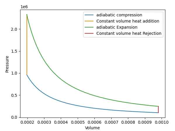
1. Adiabatic compression (1-2)- air and fuel mixture is compressed isentropically inside the cylinder.
2. Constant volume heat addition (2-3)- combustion take place inside the cylinder due to external source.
3. Adiabatic expansion (3-4) - high pressure and high temperature gases expand isentropically inside the cylinder.
4. Constant volume heat rejection (4-1):- gases come out from the cylinder and cycle is completed.

we have to give required inputs and by using basic thermodynamic formulas type in the code and save the required output. and to make a adiabatic curve by using the calling the function .

Adiabatic Curve is attain by using term 'v/v_c',

v = 1+(0.5*(cr-1)*(R+1-cos(theta)-(R^2-sin^2 theta)^0.5))*v_c//

Description:

• In this Program code we are using this adiabatic curve eqn as Function to attain curve plots at expansion and Compression.
• Initially, we are giving some inputs such as Initial Pressure,Temperature and Gamma Value. Also we Mention Heat Addition Temperature with engine geometric parameters.
• Then,Calculating volume,pressure & Temperature at various state points.
• By using these State point variable construct the PV Diagram.

SOLUTION PROCEDURE:

Step 1: Creating an Function to Attain adiabatic curve eqn as Function to attain curve plots at expansion and Compression.

v = 1+(0.5*(cr-1)*(R+1-cos(theta)-(R^2-sin^2 theta)^0.5))*v_c//

Step 2: Generating Default Inputs for Otto Cycle Such As Initial Pressure,Temperature and Gamma Value. Also we Mention Heat Addition Temperature.

# inputs
# initial Pressure
p1 = 101325
# initial Pressure
t1 = 500
# gamma value
gamma = 1.4
# temperature at het addition
t3 = 2300

Step 3: Generating Default Inputs for Engine Geometric Parameters Such As Bore, Stroke, length of Connecting rod and Compression Ratio.

# geometric parameters
bore = 0.1
stroke = 0.1
con_rod = 0.1
cr = 5

Step 4: Calculating volume,pressure & Temperature at various state points.

Step 5: Calculating the thermal efficiency of otto cycle,

# Calculating the Thermal Efficiency:
Eff = 1 - [1/(cr^(gamma-1))]

Step 6: After Calculating All state Points finally Plot P-V Diagram.

Program Code:

"""
otto cycle simulator
"""
import math
import matplotlib.pyplot as plt
import numpy as np

def engine_kinematics(bore,stroke,con_rod,cr,start_crank,end_crank):
	a=stroke/2
	R = con_rod/a
	sc=math.radians(start_crank)
	ec=math.radians(end_crank)
	num_values = 50
	dtheta = (ec-sc)/(num_values-1)
	V=[]
	for i in range(0,num_values):
		theta = sc+i*dtheta
		term1 = 0.5*(cr-1)
		term2 = R+1-math.cos(theta)
		term3 = pow((pow(R,2) - pow(math.sin(theta),2)),0.5)
		V.append((1+term1*(term2-term3))*v_c)
	return V

# inputs
# initial Pressure
p1 = 101325
# initial Pressure
t1 = 500
# gamma value
gamma = 1.4
# temperature at het addition
t3 = 2300

# geometric parameters
bore = 0.1
stroke = 0.1
con_rod = 0.1
cr = 5

# volume Computations
v_s = (math.pi/4)*pow(bore,2)*stroke
v_c = v_s / (cr-1)
v1 = v_c + v_s


# state pt 2
v2 = v_c
# p2v2^gamma = p1v1^gamma
p2 = p1*pow(v1,gamma)/ pow(v2,gamma)
# p2v2/t2 = p1v1/t1 | rhs = p1v1/t1 | t2= p2v2/rhs
rhs = p1*v1/t1
t2 = p2*v2 / rhs

V_compression = engine_kinematics(bore,stroke,con_rod,cr,180,0)
#p_comp*v_comp^gamma = constant = p1v1^gamma
constant = p1*pow(v1,gamma)
P_compression=[]
for v in V_compression:
	P_compression.append(constant/pow(v,gamma))


# state pt 3
v3 = v2
# p3v3/t3 = p2v2/t2 | rhs = p2v2/t2 | p3=t3*rhs/v3
rhs = p2*v2/t2
p3 = rhs*t3/v3

V_expansion = engine_kinematics(bore,stroke,con_rod,cr,0,180)
#p_comp*v_comp^gamma = constant = p3v3^gamma
constant = p3*pow(v3,gamma)
P_expansion=[]
for v in V_expansion:
	P_expansion.append(constant/pow(v,gamma))


# state pt 4
v4 = v1
# p4v4^gamma = p3v3^gamma
p4 = p3*pow(v3,gamma)/ pow(v4,gamma)
# p4v4/t4 = p3v3/t3 | rhs = p3v3/t3 | t4= p4v4/rhs
t4 = p4*v4 / rhs

# calculating the Thermal Efficiency:
# eff = 1 - [1/(cr^(gamma-1))]

eff = (1- (1/(pow(cr,(gamma-1)))))*100
eff= str(eff)

print ('Thermal_Efficiency= '+eff+' %')

# Resultant PV Diagram
plt.plot(V_compression,P_compression,label='adiabatic compression')
plt.plot([v2,v3],[p2,p3],label='Constant volume heat addition')
plt.plot(V_expansion,P_expansion,label='adiabatic Expansion')
plt.plot([v4,v1],[p4,p1],label='Constant volume heat Rejection')
plt.xlabel('Volume')
plt.ylabel('Pressure')
plt.legend()
plt.savefig('PV diagram - Otto Cycle')
plt.show()

RESULTS:

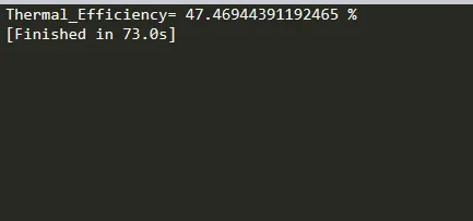
1) Output Of Thermal Efficiency:

Thus,the Thermal Efficiency of the otto cycle for the given Parameters is 47.47%//

Thermal Efficiency = 47.47%

2) P-V Diagram:

PV diagram Of the Otto cycle is plotted below,

Conclusion:

Thus,the PV Diagram of a Otto Cycle is Plotted and the Output of the Program is shown the Thermal Efficiency Of an Engine.