Week 2 Air standard Cycle

Aim:

Writing the code to create the PV diagram and finding the thermal efficiency of an engine

Research and Objective:

The physics behind the engine working is determined at four stages. There are two main parts to engine operation: the mechanical operation of the engine parts, and the thermodynamics through which the engine produce work and power. The thermodynamics allows you to design and predict engine performance.

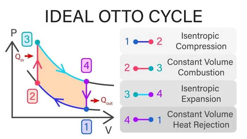
In an internal combustion engine, fuel and air are ignited inside a cylinder. The hot exhaust pushes a piston which is connected to a crankshaft to produce power. The burning of fuel is not a continuous process but occurs very quickly at regular time intervals. Between ignitions, the engine parts move in a repeated sequence called a cycle. The engine is called a four-stroke engine because there are four movements, or stroke, of the piston during one cycle. An illustration of ideal otto engine is explained in the figure below.

Governing equations:

Compression ratio `(r_c)= (V_1/V_2 ) or 1+ V_s/V_c`

Swept Volume `(V_c) = π/4. d^2.l,` where d is bore diameter and l is stroke length,

Adiabatic process equation = `p.v^γ=`constan`, where p is pressure and v is volume

Ideal gas equation `p.ν=m.R.T`, T= temperature`

`V/V_c =1+1/2 (r_c-1)[R+1-cosθ-(R^2-sin^2 θ)^(1/2)],`

where `R = 2 L_c /L`

Thermal efficiency `η=1- 1/r^(γ-1)`

where L_c is Length of the crank rod

L is stroke

r is compression ration

Body of the objective:

#Otto Cycle simulator and Engine_kinematics

import math
import matplotlib.pyplot as plt

def engine_kinematics(bore, stroke, con_rod, cr, start_crank, end_crank):
    
    # geometric parameters
    a = stroke/2
    R = con_rod/a
    
    # Volume parameters
    V_s = math.pi*(1/4)*pow(bore,2)*stroke
    V_c = V_s/(cr-1)
    
    sc = math.radians(start_crank)
    ec = math.radians(end_crank)
    
    num_values = 50
    
    dtheta = (ec-sc)/(num_values-1)
    
    V = []
    
    for i in range(0,num_values):
        theta = sc + i*dtheta
        term1 = 0.5 * (cr-1)
        term2 = R + 1 - math.cos(theta)
        term3 = pow(R,2) - pow(pow(math.sin(theta),2),0.5)
        term4 = pow(term3,0.5)
        # Formula
        V.append((1 + term1*(term2 - term4))*(V_c))
         
    return V

# inputs
p1 = 101325 # in pascals
t1 = 500 # in kelvin
gamma = 1.4
t3 = 2300 # combution temperature in kelvin

#geometric parameters
bore = 0.1 # in meters
stroke = 0.1
con_rod = 0.15
cr = 8

# Volume computation
v_s = (math.pi/4)*pow(bore,2)*stroke # swept volume
v_c = v_s/(cr-1) # compression volume
v1 = v_c + v_s

#State point 2 # clearance volume
v2 = v_c

#P2v2^gama = p1v1^gamma # pressure
p2 = p1*pow(v1,gamma)/pow(v2,gamma)

# p2v2/t2 = p1v1/t1  | rhs = p1v1/t1 | p2v2/t2 = rhs | t2 = p2v2/rhs determining temperature
rhs = p1*v1/t1
t2 = p2*v2/rhs
V_compression = engine_kinematics(bore, stroke, con_rod, cr, 180, 0)

constant = p1*pow(v1,gamma)

P_compression =[]

for v in V_compression:
    P_compression.append(constant/pow(v,gamma))
    

# State point 3
v3 = v2

#p3v3/t3 = p2v2/t2 | rhs = p2v2/t2 | p3 = rhs*t3/v3 determining pressure

rhs = p2*v2/t2
p3 = rhs*t3/v3

V_expansion = engine_kinematics(bore, stroke, con_rod, cr, 0, 180)

constant = p3*pow(v3,gamma)

P_expansion =[]

for v in V_expansion:
    P_expansion.append(constant/pow(v,gamma))
    
#State point 4
v4 = v1

#p4v4^gamma = p3v3^gamma
p4 = p3*pow(v3,gamma)/pow(v4,gamma)

#p4v4/t4 = rhs
t4 = p4*v4/rhs

#Calculating the thermal efficiency
thermal_efficiency = 1-(1/(pow(cr,gamma-1)))
print(thermal_efficiency)

plt.plot([v2,v3],[p2,p3])
plt.plot(V_compression, P_compression)
plt.plot(V_expansion, P_expansion)
plt.plot([v4,v1],[p4,p1])
plt.show()

Conclusions:

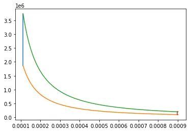
The plot was explained as shown in the image and also the thermal efficiency of the engine is 0.56473