Week 5 - Curve fitting
FAQs of Challenge:
1. What does popt and pcov mean ?
popt: array
Ans: Optimal values for the parameters so that the sum of the squared residuals of f(xdata, *popt) - ydata is minimized.
pcov: 2-D array
Ans: The estimated covariance of popt. The diagonals provide the variance of the parameter estimate. To compute one standard deviation errors on the parameters use perr = np.sqrt(np.diag(pcov)).
How the sigma parameter affects the estimated covariance depends on absolute_sigma argument, as described above.
If the Jacobian matrix at the solution doesn’t have a full rank, then ‘lm’ method returns a matrix filled with np.inf, on the other hand ‘trf’ and ‘dogbox’ methods use Moore-Penrose pseudoinverse to compute the covariance matrix.)
https://docs.scipy.org/doc/scipy/reference/generated/scipy.optimize.curve_fit.html
2. What does the np.array(temperature) do ?
Ans: np.array(temeeprature): stores the values of temeprature in array and transfers it to the function of numpy module. In this particular program it performs specific curve fit to obtain the perfect curve fitting with new co-efficients
5. What needs to be done in order to make the curve fit perfect?
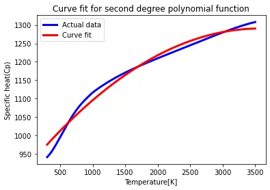
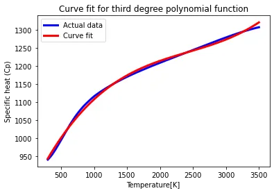
6. Show empirically as to how well your curve has been fit.
import math
import numpy as np
import matplotlib.pyplot as plt
from scipy.optimize import curve_fit

#curve fit for first degree polynomial function
def func(x,a,b):
    return a+b*x

def read_file(): # to read the theraml data file in the directory folder
    temperature = [] # Initialising empty arrays
    cp = []
    # using the for loop and open command the file called data is opened and aslo
        #by mentionting the 'r' read mode can be activated
    for line in open('data','r'):
       # to split the data seperated by ',' in the data file, as a result the array with two entities can be executed
        values = line.split (',')
       # indicating the index and conversion of the values from strings into float consisted in the text file
       # Append() coomand to add the data into empty arrays
        temperature.append(float(values[0]))
        cp.append(float(values[1]))

    return [temperature, cp]


#Main program
# to read the data in the file of the given variables in the function
temperature ,cp = read_file()
# inbulit commond to perform curvit method. 'func' parameter reperesents the mathematical equation in the program
popt, pcov = curve_fit(func, temperature,cp)
# By defining the function here , the new co-efficeints can be executed in the defined equation. '*' helps tp refer the popt co-efficients
fit_cp = func(np.array(temperature), *popt) #it performs specific curve fit to obtain the perfect curve fitting with new co-efficients

plt.plot(temperature, cp, color = 'blue', linewidth = 3)
plt.plot(temperature, fit_cp, color = 'red', linewidth = 3)
plt.legend(['Actual data', 'Curve fit'])
plt.title('Curve fit for First degree polynomial function')
plt.xlabel('Temperature[K]')
plt.ylabel('Specific heat (Cp)')
plt.show()

#curve fit  for second polynomial function
def func(x,a,b,c):
    return a+b*x+c*pow(x,2)

def read_file():
    temperature = [] # Initialising empty arrays
    cp = []
    # using the for loop and open command the file called data is opened and aslo
        #by mentionting the 'r' read mode can be activated
    for line in open('data','r'):
       # to split the data seperated by ',' in the data file, as a result the array with two entities can be executed
        values = line.split (',')
       # indicating the index and conversion of the values from strings into float consisted in the text file
       # Append() coomand to add the data into empty arrays
        temperature.append(float(values[0]))
        cp.append(float(values[1]))

    return [temperature, cp]


#Main program
# to read the data in the file of the given variables in the function
temperature ,cp = read_file()
# inbulit commond to perform curvit method. 'func' parameter reperesents the mathematical equation in the program
popt, pcov = curve_fit(func, temperature,cp)
# By defining the function here , the new co-efficeints can be executed in the defined equation. '*' helps tp refer the popt co-efficients
fit_cp = func(np.array(temperature), *popt) #it performs specific curve fit to obtain the perfect curve fitting with new co-efficients

plt.plot(temperature, cp, color = 'blue', linewidth = 3)
plt.plot(temperature, fit_cp, color = 'red', linewidth = 3)
plt.legend(['Actual data', 'Curve fit'])
plt.title('Curve fit for second degree polynomial function')
plt.xlabel('Temperature[K]')
plt.ylabel('Specific heat(Cp)')
plt.show()

#curve fit for third degree polynomial function
def func(x,a,b,c,d):
    return a+b*x+c*pow(x,2)+d*pow(x,3)

def read_file(): # to read the theraml data file in the directory folder
    temperature = [] # Initialising empty arrays
    cp = []
    # using the for loop and open command the file called data is opened and aslo
        #by mentionting the 'r' read mode can be activated
    for line in open('data','r'):
       # to split the data seperated by ',' in the data file, as a result the array with two entities can be executed
        values = line.split (',')
       # indicating the index and conversion of the values from strings into float consisted in the text file
       # Append() coomand to add the data into empty arrays
        temperature.append(float(values[0]))
        cp.append(float(values[1]))

    return [temperature, cp]


#Main program
# to read the data in the file of the given variables in the function
temperature ,cp = read_file()
# inbulit commond to perform curvit method. 'func' parameter reperesents the mathematical equation in the program
popt, pcov = curve_fit(func, temperature,cp)
# By defining the function here , the new co-efficeints can be executed in the defined equation. '*' helps tp refer the popt co-efficients
fit_cp = func(np.array(temperature), *popt) # specific fit again to obtain the perfic curve fitting

plt.plot(temperature, cp, color = 'blue', linewidth = 3)
plt.plot(temperature, fit_cp, color = 'red', linewidth = 3)
plt.legend(['Actual data', 'Curve fit'])
plt.title('Curve fit for third degree polynomial function')
plt.xlabel('Temperature[K]')
plt.ylabel('Specific heat (Cp)')
plt.show()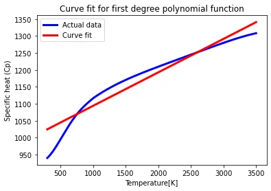
References:
Curve fitting introduction and polynomial equations:
http://citeseerx.ist.psu.edu/viewdoc/download?doi=10.1.1.397.1367&rep=rep1&type=pdf