Week 2 Air standard Cycle

AIM:-

To write a code to solve otto cycle and plot for it.using python

OBJECTIVES:-

•  writing a code to create a PV diagram
•  to calculate the thermal efficiency of the engine

THEORY:-

An Otto cycle is an idealized thermodynamic cycle that describes the functioning of a typical spark ignition piston engine. ... The Otto cycle is a description of what happens to a mass of gas as it is subjected to changes of pressure, temperature, volume, addition of heat, and removal of heat.

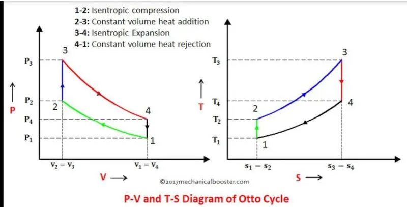
1–2, isentropic compression

2–3, constant-volume heat addition

3–4, isentropic expansion

 4–1, constant-volume heat rejection.

General relation

>1-2&3-4 compression&expansion

P.V^gamma=constant

>2-3 and 4-1 heat addition and rejection

(P/V)=constant

>Ideal gas equation

P*V/t=constant

>compression ratio 

(V_s+V_c)/V_c

change of volume inside the engine

combustion chamber:-

(V/V_c)=1+(1/2)(cr-1)(R+1-cos(theta)-(R^2-sin^2(theta))^0.5)

thermal efficiency= 1-(1/cr^(gamma-1)

sample code:-

import math
import matplotlib.pyplot as plt

def engine_kinematics(bore,stroke,connecting_rod,c_r,start_crank_angle,end_crank_angle):

#Engine geometry properties
	r=stroke/2
	n=connecting_rod/r

	#volume parameters

	v_swept = (math.pi/4)*pow(bore,2)*stroke
	v_clearance = v_swept/(c_r-1)

	theta_startcrank = math.radians(start_crank_angle)
	theta_endcrank = math.radians(end_crank_angle)

	num_val = 100
	dtheta = (theta_endcrank - theta_startcrank)/(num_val - 1)
	V=[]
	for i in range(0,num_val):
		theta=theta_startcrank + i*dtheta
		term_1 = 0.5*(c_r - 1)
		term_2 = n+1 - math.cos(theta)
		term_3 = (pow(n,2) - pow(math.sin(theta),2))
		term_3 = pow(term_3,0.5)
		V.append(1 + term_1*(term_2 -term_3)*v_clearance)
	return V


def engine_kinematics(bore,stroke,con_rod,cr,start_crank,end_crank):
	
	

	

	
	# Geometric Parameters 
	a=stroke/2
	R=con_rod/a

	# Volume Parameters
	V_s= math.pi*(1/4)*pow(bore,2)*stroke    
	V_c=V_s/(cr-1)

	sc=math.radians(start_crank)
	ec=math.radians(end_crank)

	num_values=50
	dtheta=(ec-sc)/(num_values-1)
	V=[]
	for i in range(0,num_values ):
		theta=sc+i*dtheta
		#print(theta)
		term1=0.5*(cr-1)
		term2=R+(1-math.cos(theta))
		term3=pow(R,2)-pow(math.sin(theta),2)
		term3=pow(term3,0.5)	

		V.append((1+term1*(term2-term3))*V_c)

	return V

#Input variables

gamma = 1.4
T3 = 2000

#State variable
#ambient atmospheric conditions asssumed
p1 = 101325
T1 = 350

#Egine geometry properties

bore=0.15
stroke = 0.2
connecting_rod = 0.8
c_r = 10

#calculating swept volume and clearence volume

v_swept = (math.pi/4)*pow(bore,2)*stroke
v_clearence = v_swept/(c_r-1)
v1 = v_swept + v_clearence
v2 = v_clearence

#stae variables at state point 2
#p2*v2^gamma = p1*v1^gamma

p2 = p1*pow(c_r,gamma)

#(p1*v1)/T1 = (p2*v2)/T2 = p2*v2*T1/(p1*v1)

T2 = p2*v2*T1/(p1*v1)

V_comp = engine_kinematics(bore,stroke,connecting_rod,c_r,180,0)
C_const = p1*pow(v1,gamma)
P_const = []
for v in V_comp:
	P_const.append(C_const/pow(v,gamma))

#State variables at state point 3

v3=v2

rhs=p2*v2/T2
p3=rhs*T3/v3

V_exp = engine_kinematics(bore,stroke,connecting_rod,c_r,0,180)
C_const = p3*pow(v3,gamma)
P_exp =[]
for v in V_exp:
	P_exp.append(C_const/pow(v,gamma))

#State variables at state point 4
v4=v1

p4=p3*pow(v3,gamma)/pow(v4,gamma)

T4= p4*v4*T3/(p3*v3)

plt.plot(V_comp,P_const)
plt.plot([v2,v3],[p2,p3])
plt.plot(V_exp,P_exp)
plt.plot([v4,v1],[p4,p1])
plt.ylim([-500000,8000000])
plt.xlim([0,0.005])
plt.xlabel('Volume (m^3)')
plt.ylabel('Pressure(Pa)')
plt.title('p-V diagram of an Otto Cycle')
plt.text(0.00385,-250000,r'$ 1 $')
plt.text(0.0002,2000000,r'$ 2 $')
plt.text(0.00385,400000,r'$ 3 $')
plt.grid()
plt.show()

#calculating thermal efficieny

thermal_efficiency = 1-(1/pow((c_r),(gamma-1)))
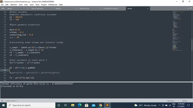
print('Thermal efficiency of given Otto Cycle is :',thermal_efficiency)

code explanation:-

1. First of all,we need to identify the variables of each point the Otto-cycle and how the volume and pressure changes from each state.
2. The initial pressure ,volume ,temperature of atmospheric air is p1,v1 and t1.
3. During Suction stroke,the inlet valve opens and teh air intake occurs and the state variable changes from p1v1 to p2v2.After the intake process the inlet valve closes,Compression stroke takes place during this stroke the charge compressed the state variable changes from p2v2 to p3v3.After the compression process Power stroke takes place the state variables change from p3v3 to p4v4 then exhaust stroke the exhaust stroke the exhaust valve opens and the burned gas is expelled the state variables from p4v4 to p1v1
4. Then the state variables are calculated using thermodynamc relations of each process.
5. Since the state change from p2v2 to p3v3 is not linear we havee to create the curve that relates to the process.In order to acheive theta,the code has a function call with function name"engine_kinematics" this function call is done for creating the curve of adiabatic compression and adiabatic expansion process process which they are not a straight line.With function call and thermodynamics relation,the v_compression and v_expansion are calculated.
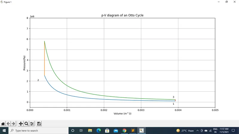
6. After calculating the values of the state variable use matplotlib(_) to plot the pv diagram of the otto cycle.pltshow() commands is used to display the plot.
7. Add labels for axis ad give a title to the pv diagram by using plt.xlabel('_').plt.ylabel('_') 

output:-

conclusion:-

p-v diagram of otto cycle is obtained.

thermal efficiency is 60%