Project 2 - Rankine cycle Simulator
AIM:-
writing a code to simulate rankine cycle
OBJECTIVES:
- To simulate rankine cycle
- Extracting steam and water properties
- calculating all the state points
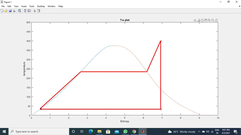
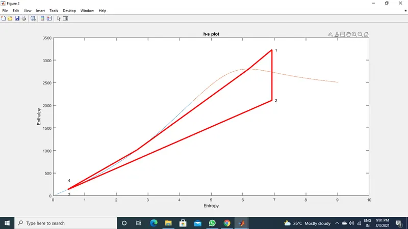
- plotting the T vs S and Hvs S
THEORY:-
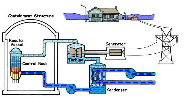
The Rankine cycle or Rankine Vapor Cycle is the process widely used by power plants such as coal-fired power plants or nuclear reactors. In this mechanism, a fuel is used to produce heat within a boiler, converting water into steam which then expands through a turbine producing useful work
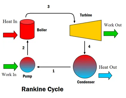
1-2:Isentropic compression in pump
2-3:constant pressure heat addition in boiler
3-4:Isentropic expansion in turbine
4-1:constant pressure and heat rejection in condenser
The steps in the Rankine Cycle as shown in Figure
- Pump: Compression of the fluid to high pressure using a pump
- Boiler: The compressed fluid is heated to the final temperature (which is at boiling point), therefore, a phase change occurs—from liquid to vapor.
- Turbine: Expansion of the vapor in the turbine.
- Condenser: Condensation of the vapor in the condenser
clear all
close all
clc

disp('Rankine cycle simulator')
disp('process 1-2:Isentropic expansion in turbine')
disp('process 2-3:constant pressure and heat rejection in condenser')
disp('process 3-4: Isentropic compression in pump')
disp('process 4-1:constant pressure heat addition in boiler')

% getting the initial data inputs
% t1=input('Enter the turbine inlet temp: ');
% p1=input('Enter the turbine inlet pressure: ');
% p2=input('Enter the turbine outlet pressure: ');
t1 = 400;
p1 = 30;
p2 = 0.05;

% state_1 parameters(turbine inlet)
tsat=XSteam('Tsat_p',p1);
h1=XSteam('h_pt',p1,t1);
s1=XSteam('s_pt',p1,t1);

% state_2parameter (condenser inlet)
s2=s1;
sf2=XSteam('sL_p',p2);
sg2=XSteam('sv_p',p2);
% s2=sf2+(X2*sfg2)
 X2=(s2-sf2)/(sg2-sf2);  %dryness_fraction

 t2=XSteam('T_ps',p2,s2);
 h2=XSteam('h_px',p2,X2);
 hf2=XSteam('hL_p',p2);

%  state 3parameters (pump inlet)
p3=p2;
t3=t2;
s3=sf2;
h3=hf2;
t5=tsat;

% state 4  parameters (boiler inlet
s4=s3
p4=p1
h4=XSteam('h_ps',p4,s4);
cp=XSteam('cp_ps',p4,s4);
cv=XSteam('cv_ps',p4,s4);
c=cp/cv;
t4=t3*((p4/p3)^(c-1)/c)

% state_5,6
t5=tsat;
h5=XSteam('hL_p',p1);
s5=XSteam('sL_p',p1);
t6=t1;
h6=XSteam('hV_p',p1);
s6=XSteam('sV_p',p1);

% plotting T_S diagram
t=linspace(5,400,50000)
for i=1:length(t)
    s(i)=XSteam('sL_t',t(i));
    S(i)=XSteam('SV_t',t(i));
    h(i)=XSteam('hL_t',t(i));
    H(i)=XSteam('hV_t',t(i));
end
figure(1)
plot(s,t);
hold on
plot(S,t);

plot([s1,s2,s3,s4,s5,s6],[t1,t2,t3,t4,t5,tsat],'linewidth',3,'color','r');
hold on
plot([s6,s1],[tsat,t1],'linewidth',3,'color','r')


% %  to plot above the saturated temperature
% a=linspace(tsat,t1,500);
% for i=1:length(a)
%     d(i)=XSteam('s_pt',3,'color','r')
% end
% plot(d,a,'linewidth',3,'color','r')
 title('T-s plot')

axis([0 10 0 500])
text(s1,t1,'1')
text(s2,t2,'2')
text(s3,t3,'3')
text(s4,t4,'4')


xlabel('Entropy')
ylabel('temperature')

figure(2)
plot(s,h);
hold on
plot(S,H);
plot([s1,s2,s3,s4,s5,s6,s1],[h1,h2,h3,h4,h5,h6,h1],'linewidth',3,'color','r');
title('h-s plot')
text(s1+0.1,h1,'1')
text(s2+0.1,h2,'2')
text(s3,h3-100,'3')
text(s4,h4+200,'4')

xlabel('Entropy')
ylabel('Enthalpy')
% workdone by the turbine
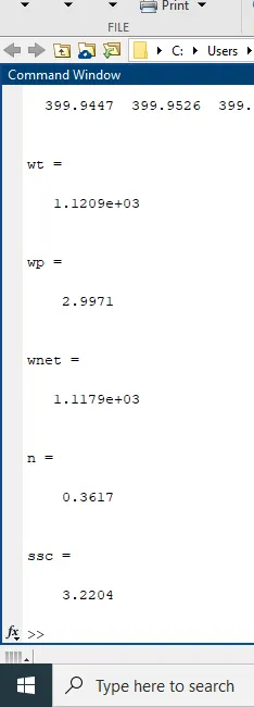
wt=h1-h2
% workdone by the pump
wp=h4-h3

% net workdone
wnet=wt-wp

% heat supplied
q=h1-h4;

% effiency
n=wnet/q
%  specific steam consumption

ssc=3600/wnet
CODE EXPLANATION:
- Initially give the given inputs
- calculating state points by XSteam
- XSteam data is used to extract steam and water propertis of entropy,enthalpy,temperatures and vapour conditions
- ploting of T vs s in figure(1)
- ploting of h vs s in figure(2)
- calculating workdone by turbine , pump,net workdone ,heat supplied ,effiency,specific heat consumption
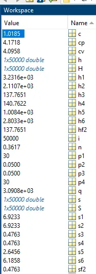
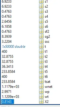
Out puts: