Week 2 Air standard Cycle

Air Standard Cycle - Otto Cycle:

• Otto Cycle is a set of process used by SI(spark ignition engines). These engines might be 2 stroke or 4 stroke.
• These engines work by a) getting the charge(air fuel mixture) in cylinder as intake, b) compress the charge, c)igniting the mixture using a spark, converting chemical energy into thermal energy,d) causing the mixture to expand,e) exjecting the combustion products and replace them with a new charge and repeat the process.

 Processes in otto cycle:

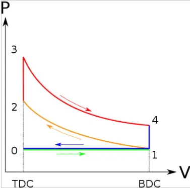
• Intake stroke, gasoline vapor and air drawn into engine. (0->1)
• Isentropic Compression stroke. (1->2)
• Combustion (spark), short time, essentially constant volume. (2->3)
• Power stroke: Isentropic expansion. (3->4)
• Valve exhaust: valve opens, gas escapes.
• Rejection of heat at constant volume. (4->1)
• Exhaust stroke, piston pushes remaining combustion products out of chamber. (1->0)

Terminology for Otto Cycle:

Compression Ratio: It is defined as the ratio of volume before and after compression.

Compression Ratio (cr) = `(V_s+V_c)/V_c`

Vs is swept volume

Vc is clearance volume

Also, V1 = Vs+Vc and V2 = Vc.

Therefore, Compression Ratio can be calculated using V1/V2.

Swept Volume: The volume through which a piston moves as it makes a stroke.

Clearance Volume: The volume between the cylinder head and the piston when the piston is at TDC.

Thermal Efficiency: `eta_(th) = 1- (T_4-T_1)/(T_3-T_2) = 1-1/(cr^(gamma-1))`.

Engine Parameters:

• Bore Diameter = 0.1m
• Stroke Length = 0.1m
• Connecting rod length = 0.15m
• Compression ratio = 12.

Inputs:

Gamma = 1.4

State variables at 1:

P1 = 10135 N/m^2

T1 = 500 K

State variables at 3:

T3 = 2300K

import math
import matplotlib.pyplot as plt

def engine_kinematics(bore, stroke, con_rod, cr, start_crank, end_crank):
    # Geometric parameters
    a = stroke/2
    R = con_rod/a
    # Volume parameters
    V_s = math.pi* (1/4) *pow(bore,2)*stroke
    V_c = V_s/ (cr-1)

    sc = math.radians(start_crank)
    ec = math.radians(end_crank)
    num_values = 100
    dtheta = (ec-sc) / (num_values-1)
    V = []

    for i in range(0,num_values):
        theta = sc+i*dtheta
        term1 = 0.5*(cr-1)
        term2 = R + 1-math.cos(theta)
        term3 = pow(R,2) - pow(math.sin(theta),2)
        term3 = pow(term3,0.5)
        V.append((1 + term1*(term2-term3))*V_c)
    return V

# inputs
p1 = 101325
t1 = 500
t3 = 2300
gamma  = 1.4

# geometric parameters
bore = 0.1
stroke = 0.1
con_rod = 8.15
cr = 12

# Volume computation
V_s = (math.pi/4)*pow(bore, 2)*stroke
V_c = V_s/(cr-1)
v1 = V_c + V_s

# state point 2
v2 = V_c

# p2v2^gamma = p1v1^gamma
p2 = p1*pow(v1/v2,gamma)
# p2v2/t2 = p1vi/t1 | rhs = piv1/t1 | p2v2/t2 = rhs | t2 = p2v2/rhs
rhs = p1*v1/t1
t2 = p2*v2/rhs

V_comp = engine_kinematics(bore, stroke, con_rod, cr, 180,0)
const = p1*pow(v1,gamma)
P_comp = []
for v in V_comp:
    P_comp.append(const/pow(v,gamma))

# state point 3
v3 = v2
#pv/t (rhs) is constant
p3 = rhs*t3/v3

V_expan = engine_kinematics(bore, stroke, con_rod, cr, 0, 180)
const = p3*pow(v3,gamma)
P_expan = []
for v in V_expan:
    P_expan.append(const/pow(v,gamma))

# state point 4
v4 = v1
#p4v4^ gamma = p3v3^gamma
p4 = p3*pow(v3, gamma)/pow(v4, gamma)
t4 = p4*v4/rhs

#Thermal Efficiency 
T_eff = (1-(1/pow(cr,gamma-1)))*100
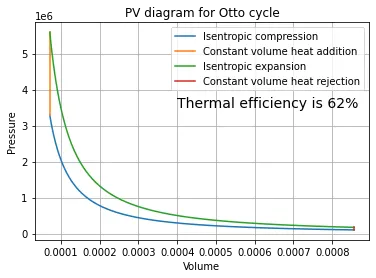
st = 'Thermal efficiency is ' + str(math.trunc(T_eff)) + '%'

#plotting
plt.plot(V_comp,P_comp, label = 'Isentropic compression')
plt.plot([v2, v3], [p2,p3], label = 'Constant volume heat addition')
plt.plot(V_expan, P_expan, label = 'Isentropic expansion')
plt.plot([v4,v1],[p4,p1], label = 'Constant volume heat rejection')
plt.text(0.0004,3.5*pow(10,6), st, fontsize = 14)
plt.xlabel('Volume')
plt.ylabel('Pressure')
plt.title('PV diagram for Otto cycle')
plt.grid()
plt.legend()
plt.show()

Plot: