Week 2 Air standard Cycle

AIM:

Write code that can solve an otto cycle and make plots for the same, based on the concepts that we have learnt during the forward kinematics routine. Also provide the following for the assignment:

1. Code should plot a PV diagram for this cycle (Otto)
2. Print the thermal efficiency for the same.

THEORY:

The topics, keywords and concepts revelant for this assignment are explained below:

• Otto Cycle : This cycle is also known as petrol cycle, is an idealized thermodynamic cycle that describes the functioning of a typical spark ignition piston engine. It is the most common thermodynamic cycle found in automobile engines. It is basically the description of what happens to a mass of gas as it is subjected to changes of pressure, temperature, volume, heat addition, and removal of heat. The mass of the gas that is subjected to those changes is called the system. The system, in this case, is defined to be the fluid (gas) within the cylinder. By describing the changes that take place within the system, it will also describe in inverse, the system's effect on the environment. In the case of the Otto cycle, the effect will be to produce enough net work from the system so as to propel an automobile and its occupants in the environment.
  The Otto cycle is constructed from:
  • Top and bottom of the loop: a pair of quasi-parallel and isentropic processess (frictionless, adiabatic reversible).
  • Left and right sides of the loop: a pair of parallel isochoric processses (constant volume).
    
    
• Forward Kinematics : This refers to the use of the kinematic equations of the robot to compute the position of the end-effector from the specified values for the joint parameters. The kinematic equations of the robot are used in robotics, computer games and animation. The reverse process that computes the joint parameters that achieve the specified position of the end effector is known as inverse kinematics.
  
  
• Thermal Efficiency : In thermodynamics, the thermal efficiency is a dimensionless performance measure of a device that uses thermal energy, such as an internal combustion engine, a steam turbine or steam engine, a boiler, furnace, or a refrigerator for example.
  In general, the thermal efficiency, `eta_(th)`, of any heat engine is defined as the ratio of the work it does, W, to the heat input at the high temperature, `Q_H`.
  `eta_(th) = W/Q_H`
  It represents the fraction of heat, `Q_H` that is converted to work. Since energy is conserved according to the first law of thermodynamics and energy cannot be converted to work completely, the heat input, `Q_H`, must equal the work done, W, plus the heat that must be dissipated as waste heat, `Q_C` into the environment. Therefore we can rewrite the formula for thermal efficiency as:
  `eta_(th) = W/Q_H = (Q_H - Q_C)/Q_H = 1 - Q_C/Q_H`
  The heat absorbed occurs during the combustion of fuel-air mixture, when the spark occurs, roughly at constant volume. Since during an isochoric process there is no work done by or on the system, the first law of thermodynamics dictates: `DeltaU = DeltaQ`. Therefore the heat rejected and added are given by:
  `Q_(add) = mc_v(T_3 - T_2)`
  `Q_(out) = mc_v(T_4 - T_1)`
  Substituting these values results in the thermal efficiency yields:
  `eta_(th) = 1 - (T_4 - T_1)/(T_3 - T_2)`
  We can simplify the above expression using the fact that the processes `1 to 2` and `3 to 4` are adaibatic and for an adiabatic process the following p, V, T formula is valid:
  `[V_2/V_1]^(gamma) = [T_1/T_2]^(gamma/(gamma-1))`
  It can be derived that,
  `(T_4 - T_1)/(T_3 - T_2) = (V_2/V_1)^(gamma-1)`
  In this equation, the ratio `V_2/V_1` is known as the compression ratio, `r_c`. When we rewrite the expression for thermal efficiency using the compression ratio, we conclude the air standard Otto Cycle thermal efficiency is a function of compression ratio and `gamma = C_p/C_v`.
  `eta_(th) = 1 - (T_4 - T_1)/(T_3 - T_2) to eta_("otto") = 1 - (V_2/V_1)^(gamma -1) = 1 - 1/(r_c^(gamma -1))`
  
  
• Compression Ratio (`r_c`) : The compression ratio is the ratio between the volume of the cylinder and combustion chamber in an internal combustion engine at their maximum and minimum values.
  A fundamental specification for such engines, it is measured two ways: the static compression ratio, calculated based on the relative volumes of the combustion chamber and the cylinder when the piston is at the bottom of its stroke, and the volume of the combustion chamber when the piston is at the top of its stroke.
  The dynamic compression ratio is a more advanced calculation which also takes into account gasses entering and exiting the cylinder during the compression phase.
  The formula for compression ratio is given as:
  `r_c = (V_s + V_c)/V_c`
  where, `V_s` is the swept volume and
  `V_c`is the clearance volume.
  
  
• Swept Volume (`V_s`) : This is the volume inside the cylinder displaced by the piston from the beginning of the compression stroke to the end of the stroke. This can be estimated by the cylinder volume formula: `V_s = pi/4b^2s`
  where, b is the cylinder bore (diameter) and
  s is the piston stroke length.

CODING APPROACH:

Here, we will first import all the necessary modules (in this case, matplotlib for plotting pV diagram and math for performing calculations and recognizing certain mathematical expressions such as trignometric expressions for example). After this, we will need to define a function engine kinematics. The purpose of this function is to evaluate the volume trace which will further basically provides the values for the processes `1 to 2` and `3 to 4` curve from the pV diagram for Otto Cycle.

Along with this we also need to calculate the state values using the isentropic equation and ideal gas equations etc. These values, apart from plotting the pV diagram, are also used to calculate the constant from the isentropic equations which will be used to evalute the pressure for these isentropic processes using the volume calculated from the engine kinematics function.

For this purpose a different formula is used and is given below:

`V/V_c = 1 + 1/2(r_c - 1)[R + 1 - costheta - (R^2 - sin^2theta)^(1/2)]`
where, a = stroke/2
R = (connecting rod)/a

CODE:

import matplotlib.pyplot as plt
import math

# Inputs
p1=101325 # Pascal or 1 bar
t1=500 #K
gamma=1.4
t3=2300

# dimensions of the combustion system (piston-Cylinder arrangement)
bore=0.1 #m
stroke=0.1
con_rod=0.15
c_r=12
a=stroke/2
R=con_rod/a

# Volume Parameters
V_s=(math.pi/4)*(pow(bore,2)*stroke)
V_c=V_s/(c_r-1)
v1=V_c+V_s


def engine_kinematics(bore,stroke,start_crank,end_crank):
	sc=math.radians(start_crank)
	ec=math.radians(end_crank)
	num_values=50
	dtheta=(ec-sc)/(num_values-1)
	V=[]
	for i in range(0,num_values):
		theta=sc+i*dtheta
		term1=0.5*(c_r-1)
		term2=R+1-math.cos(theta)
		term3=pow(pow(R,2)-pow(math.sin(theta),2),0.5)
		V.append((1+term1*(term2-term3))*V_c)

	return V


# At state 2,
v2=V_c
# Since, p2v2^gamma=p1v1^gamma
p2=(p1*pow(v1,gamma)/pow(v2,gamma))
# Using ideal gas equations,
rhs=p1*v1/t1 # This value remains const irrespective of the stage in the cycle
t2=p2*v2/rhs

V_compression=engine_kinematics(bore,stroke,180,0)

const=p1*pow(v1,gamma)
P_compression=[]
for v in V_compression:
	P_compression.append(const/pow(v,gamma))

#At stage 3,
v3=v2
p3=rhs*t3/v3

constant=p3*pow(v3,gamma)
V_expansion=engine_kinematics(bore,stroke,0,180)
P_expansion=[]
for v in V_expansion:
	P_expansion.append(constant/pow(v,gamma))

# At stage 4,
v4=v1
p4=(p3*pow(v3,gamma))/pow(v4,gamma)
t4=p4*v4/rhs

# Since thermal efficiency is given by: n_th = 1 - 1/(c_r^(gamma-1))
print((1 - 1/pow(c_r,(gamma-1)))*100)
plt.plot([v2,v3],[p2,p3])
plt.plot(V_compression,P_compression)
plt.plot(V_expansion,P_expansion)
plt.plot([v4,v1],[p4,p1])
plt.xlabel("Volume (V)")
plt.ylabel("Pressure (P)")
plt.title("PV diagram for Otto Cycle")
plt.show()

RESULTS:

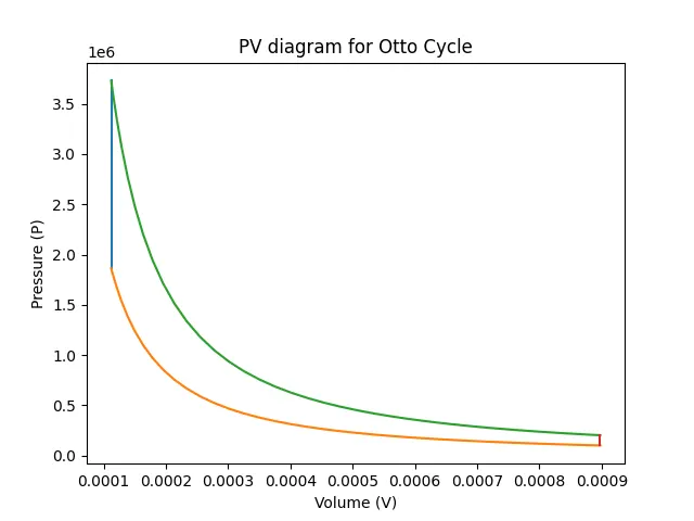
Here, first of all, the thermal efficiency of the engine system under study is approximately 56.5%. And the pV diagram obtained is as shown below:

i). For compression ratio (`r_c`) 12, we get the plot as shown below,

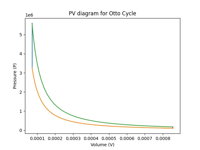
ii). Similarly for compression ratio as 8, we get to see a more clearer pV diagram for Otto Cycle: