Project:-- Creation of simulation of Otto-Cycle by PYTHON.

Aim of the project:-- Making a programe by PYTHON, which 1) gives state varriables of all states of an Otto-cycle 2) plots P-V diagram & 3) calculates thermal efficiency. The programe does all these, with the help of specific inputs given, when run.

Otto-Cycle:-- This cycle was devised by a Frenchman Beau-de-Rochas. The first engine working on this cycle was sucessfully built by German engineer A.Otto. This an idealized thermodynamic cycle & petrol engine (spark ignition) run on this cycle. Ideal otto-cycle consists of two reversible adiabetic or isentropic process & two constant volume processes as shown in the below P-V diagram. Otto Cycle also known as Constant Volume Cycle. Air is taken as working substance for Otto Cycle.

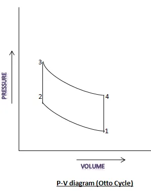
As shown in the above P-V diagram, 1-2 is reversible adiabetic compression process, 2-3 is constant volume heating process(heat additon) , 3-4 is reversible adiabetic expansion process & 4-1 is constant volume cooling process (heat rejection).

If we link this Otto cycle with runing of petrol engine(IC engine), we can say that, in the process 1-2(reversible adiabetic compression ) the piston of engine compresses the air fuel mixture & the piston moves from BDC(Bottom Dead Centre) to TDC(Top Dead Centre) of engine cylinder. So in this process, pressure & temperature increases & volume decreases but the entropy remains constant so no heat enters into or comes out from the system. So at the state point-1 the piston is at BDC & at state point 2 the piston is at TDC.

In the process 2-3, the combustion of air fuel mixture with the help of spark plug is occured at constant volume & here pressure, temperature & entropy increases.

In the process 3-4 (reversible adiabetic expansion) of the otto_cycle, expansion of working substance in side the cylinder is occured, in other words the volume inside the combustion chamber increases. Here pressure & temperature of working substance inside cylinder decreses but entropy remains constant so no heat enters into or comes out from the system. Here piston moves from TDC to BDC. This is the working stroke or power stroke of the engine.

The 4-1 process is idealized heat rejection process at constant volume. Here piston is momentarily rest at BDC. Working gas pressure drops at constant volume & heat is rejected to surrounding air.

In case of 4 stroke petrol engine additional two process are there which are intake of air & exhaust of burnt gas.

Equations Required are listed below.

1) P V^gama= constant : This is the equation shows relation between pressure & volume for adiabetic process.

2) PV/T= constant : Ideal gas equation

P= Pressure of gas; V= Volume of gas; T= Temperature of gas; gama=Cp/Cv where Cp& Cv are specific heat of gas at constant pressure & constant volume respectively.

3) V_s=(Pi/4).(bore^2).(stroke_length): V_s = Swept volume or stroke Volume, which is the volume sweept by piston in the engine cylinder in a single stroke.

4) V_c=V_s/(cr-1) : V_c = Clearance volume, which is volume occupied by working fluid when the piston ia at TDC(Top Dead Centre). cr = compression ratio, cr=(V_s+V_c)/V_c

4) V/ V_c = 1+0.5(cr-1)[R+1-cos(theta)-(R^2 - sin(theta)^2)^0.5]; This equation describes the relation between crank angle & volume inside the combustion chamber. If we solve the equation we will get the 'Volume trace'. Here V= volume inside the combustion chamber, theta= crank angle, V_c=clearance volume, R=con_rod/a, con_rod= length of connecting rod, a=crank pin radious=stroke_length/2

5) Thermal efficiency= 1-(1/cr)^(gama-1)= 1-t1/t2 = 1-t4/t3

Now a programe is to be made in Python to find out values of all state varriables (pressure, volume & temperature for the state points 1,2,3 & 4 of the Otto cycle) with some specific inputs & plotting of P_V diagram of the the Otto cycle.

The relevent code in PYTHON is given below:-

import math
import matplotlib.pyplot as plt
import numpy as np


def Engine_kinematics(bore,stroke,con_rod,cr,start_crank,end_crank):

	#Geometric parameter
	a=stroke/2
	R=con_rod/a

	# Volume parameter
	V_s=(math.pi/4)*pow(bore,2)*stroke
	V_c=V_s/(cr-1)


	theta=np.linspace(math.radians(start_crank),math.radians(end_crank),180)
	#print(theta)
	V=[]

	for i in theta:
		term1=0.5*(cr-1)
		term2=R+1-(math.cos(i))
		term3=pow(R,2)-(pow(math.sin(i),2))
		term4=pow(term3,0.5)
		V.append((1+term1*(term2-term4))*V_c)
	return(V)

# input
gama = 1.4
p1=101325  # in pascal
t1=500     # in kelvin
t3=2300    # in kelvin

# Geometric parameter

bore=0.1   
stroke=0.1
con_rod=0.15
cr=8

# Volume computation

V_s=(math.pi/4)*pow(bore,2)*stroke
V_c=V_s/(cr-1)

v1=V_s+V_c
print('Pressure at state point 1 : p1=',p1,'pascal (given as input)')
print('Volume at state point 1 : v1=', v1,'m3')
print('Temperature at state point 1 : t1=', t1,'kelvin  (given as input)')

# State point 2

v2=V_c


# p1*v1^gama=p2*v2^gama
p2=p1*pow(v1,gama)/pow(v2,gama)


#p1v1/t1=p2v2/t2=const
const=(p1*v1)/t1
t2=(p2*v2)/const

V_comp=Engine_kinematics(bore,stroke,con_rod,cr,180,0)

"""
Here elementwise operation has been done by numpy module to get P_comp

"""
con1=p1*pow(v1,gama)
P_comp=con1/pow(np.array(V_comp),gama)



print('Presssure at state point 2 : p2=',p2,'pascal')
print('Volume at state point 2 : v2=', v2,'m3')
print ('Temperature at state point 2 : t2=',t2,'kelvin')


# State point 3

v3=v2

#p3v3/t3=p2v2/t2=const
const=(p2*v2)/t2
p3=(const*t3)/v3



print ('Pressure at state point 3 : p3=',p3,'pascal')
print('Volume at state point 3 : v3=',v3,'m3')
print('Temperature at state point 3 : t3=',t3,'kelvin (given as input)') 

# State point 4

v4=v1

# p4*v4^gama=p3*v3^gama
p4=(p3*pow(v3,gama))/pow(v4,gama)

#p3v3/t3=p4v4/t4=const
const=(p3*v3)/t3
t4=(p4*v4)/const

V_exp=Engine_kinematics(bore,stroke,con_rod,cr,0,180)
con2=p3*pow(v3,gama)
P_exp=[]
for v in V_exp:
	P_exp.append(con2/pow(v,gama))


Thermal_Efficiency = 1-1/pow(cr,(gama-1))
#Thermal_Efficiency2 = 1-(t1/t2)
#Thermal_Efficiency3 = 1-(t4/t3)

print('Pressure at state point 4 : p4=', p4,'pascal')
print('Volume at state point 4 : v4=', v4,'m3')
print('Temperature at state point 4 : t4=',t4,'kelvin')	

print('Thermal Efficiency = ',Thermal_Efficiency)

# Plotting
plt.plot(V_comp,P_comp)
plt.plot([v2,v3],[p2,p3])
plt.plot(V_exp,P_exp)
plt.plot([v4,v1],[p4,p1])
plt.xlim([0,0.001])
plt.ylim([-500000,4500000])
plt.xlabel('Volume(m3)')
plt.ylabel('Pressure(Pa)')
plt.text(0.0009,-200000,'$ 1 $')
plt.text(0.0009,300000,'$ 4 $')
plt.text(0.00008,1862269,'$ 2 $')
plt.text(0.00008,3728760,'$ 3 $')
plt.title('P-V diagram of an Otto Cycle')
plt.grid()
plt.show()

Explanation of code:--

1) Import of required module: Math module is importated for methametical calculation, matplotlib.pyplot for plotting P-V diagram & numpy is imported for element wise operation on matrix.

2) The function 'Engine_kinematics is defined. The function does the operation of calculating the values of volume for the intermediate points between state points 1,2 and 3,4 that is for adiabetic expansion & adiabetic compression respectively. The function gives true nature for the curve 1-2 & 3-4.

At the point of declaration of the function, input varriables are declared which are bore-dia, stroke-length, length of connecting rod, strat crank angle (at starting of adiabetic process) & end crank angle (at the end of the adiabetic process).

Vrriables a & R are defined.

Formula for calculating swept volume (V_s) & Clearance volume (V_c) are set.

'theta' matrix has been defined with the help of linspace comand which is in the numpy module.The linspace command devides the range from start crank angle to end crank angle into 180 parts & forms the 'theta' matrix. 'theta' is the cranak angle.

After that 'V ' matrix is defined. This varriable represents the volume of working substance inside cylinder during adiabetic compression & expansion.

Here a for loop is used to append the V-matrix by using the formula for calculating volume-trace as described in the point-4 of the section 'Required Equation' above. The equation is divided in to 4 parts (term1, term2, term3, term4) to avoid complexity. Then the code 'return(V)' is used inside the function to get the value of V when the function is called.

3) Some inputs are given to the programe to calculate the state points varriables. These are gama, pressure(p1) & temperature(t1) of state point-1 & temperature (t3) of state point-3.

4) Values of some geometric parameters are declared which are bore dia, stroke length, length of connecting rod, compression ratio.

5) Sweept volume(V_s) & Clearance volume(V_c) are calculated. Volume at state point1 (v1) is the summation of V_s & V_c because at the state point 1, the piston is at BDC.

6) For state point 2, v2 is taken as V_c because at this moment the piston is at TDC. p2 is calculated by the help of equation pv^gama=constant because the 1-2 is an adiabetic compression process. t2 is calculated by ideal gas equation pv/t=constant. Besides this for getting the vaues of volumes (V_comp) in between state poins 1 & 2 (i.e. on the path 1-2) the function 'Engine_kinematics is called. The values of P (P_comp) corresponding to the values of V (V_comp) are ontained with the formula pv^gama=constant & here 'numpy' module is used for elementwise operation on the matrix V_comp.

7) For the state point 3, v3 should be equal to v2 as 2-3 is a constant volume process. t3 is given as input. p3 is obtainted applying equation pv/t=constant.

8) For state point 4, the volume v4 is equal to v1 as 4-1 is a constant volume process. p4 is obtained by applying equation pv^gama=constant as 3-4 is an adiabetic expansion process. Here also the volumes in between state points 3 & 4 are obtained by calling the function Engine _kinematics & corresponding values of pressure are calculated by using a for_loop.

9) Thermal efficiency of the Otto_cycle is calculated.

10) Values of state varriables of all the state points are also printed as part of the program.

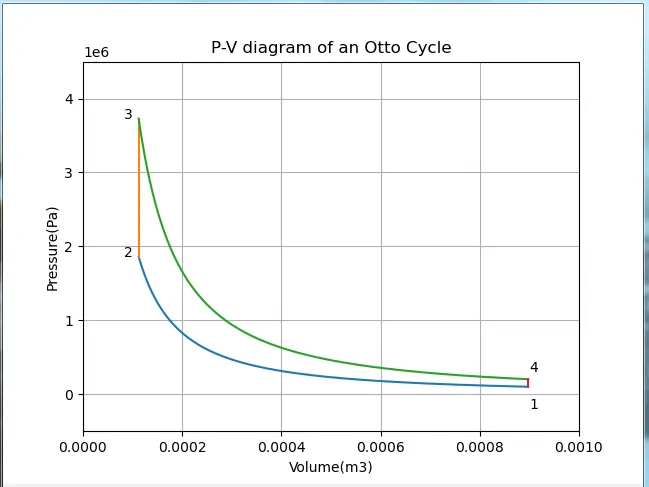
11) The plotting of the P-V diagram is done by using matplotlib.pyplot module.

Out put of the program are given below.

P-V diagram:--

Values of state varrables & Thermal Efficiency of the Otto-Cycle:--

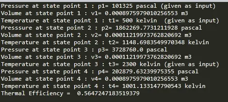
Thermal Efficiency of the Otto Cycle is =0.56 or 56%.