Otto Cycle Simulation using Python

*NOTE: The various formulae used couldn't be entered here, so the entire report has also been attached as a word document*

Aim: To write program in python to plot PV diagram for Otto Cycle and output thermal efficiency for that engine.

Theory & Governing Equations:

• The Ideal Gas Equation, it is used a lot in the program and analysis of the Otto Cycle in general.

where,

= Pressure at state “t”

= Volume at state “t”

= Temperature at state “t”

• The Otto cycle has 4 different state points consisting of 4 different processes. The processes are 1-2: Adiabatic compression, 2-3: Isochoric heat addition, 3-4: Adiabatic expansion, 4-1: Isochoric heat rejection, assuming 1, 2, 3, 4 to be 4 different state points.

The Adiabatic processes; 1-2 and 3-4 being isentropic processes are related with following equation:

where,

= Gamma (ratio of specific heats)

is assumed to be 1.4 in this case

= Pressure at state “t”

= Volume at state “t”

• The Thermal efficiency of the Otto Cycle is given by:

where,

= efficiency

= compression ratio

= Gamma

• Formula for Volume in adiabatic process:

Clearance Volume

Objectives:

• To writeprogram in python create a PV diagram of Otto Cycle of an engine.
• To output the thermal efficiency of the given engine.

Body of the Contents:

Python was the language used to code the following program.

Programs:

Engine Kinematics Function:

#Engine Kinematics
def engine_kinematics(bore, stroke, con_rod, cr, start_crank,end_crank):

	# Geometric parameters 

	a = stroke/2   #crank pin radius
	R = con_rod/a 

	#Volume Parameters 
	v_s = (math.pi/4) * pow(bore,2)*stroke  #swept volume
	v_c = (v_s)/(cr - 1)                    #clearance volume



	sc = math.radians(start_crank)    #start angle of crack converted to radians
	ec = math.radians(end_crank)      #end angle of crack converted to radians

	num_values = 50    #Number of data points to be plotted for each adiabatic process

	dtheta = (ec - sc)/(num_values-1)

	V = []

	for i in range(0,num_values):
		theta = sc + i*dtheta                #getting the different crank angles
		#Formula for Volume is split into 3 parts for ease of calculation
		term1 = 0.5*(cr - 1)                
		term2 = R + 1 - math.cos(theta)
		term3 = pow(pow(R,2) - pow(math.sin(theta),2),0.5)

		V.append((1 + term1*(term2 -term3))*v_c)

	return V

The values of bore, stroke length, connecting rod length, compression ratio, starting crank angle, ending crank angle are passed as arguments into the function.

The crank pin radius is found using stroke length value and another constant is defined uing crank pin radius and connecting rod values.

Swept Volume is calculated using bore diameter and stroke length, Clearance volume is then calculated using Swept Volume and compression ratio.

“dtheta” was calculated as the difference between starting “sc” and ending crank “ec” angles divided by the “num_values” (number of data points required). “V” Volume was initialised as an empty array.

Using a for loop, The Value of theta was increased for each iteration from starting crank angle to ending crank angle by adding “dtheta” each time. The Volume for each angle was calculated by the previously mentioned equation but due to it’s complicated nature, to avoid mistakes it was split into 3 separate terms and each of the were separately calculated and appended to “V” at the end together.

The array “V” with all the values of Volume for the data points was returned at the end of the function outside the previous for loop.

Full Program:

#Otto Cycle Simulator 

#importing required modules
import math
import matplotlib.pyplot as plt 

#Engine Kinematics
def engine_kinematics(bore, stroke, con_rod, cr, start_crank,end_crank):

	# Geometric parameters 

	a = stroke/2   #crank pin radius
	R = con_rod/a 

	#Volume Parameters 
	v_s = (math.pi/4) * pow(bore,2)*stroke  #swept volume
	v_c = (v_s)/(cr - 1)                    #clearance volume



	sc = math.radians(start_crank)    #start angle of crack converted to radians
	ec = math.radians(end_crank)      #end angle of crack converted to radians

	num_values = 50    #Number of data points to be plotted for each adiabatic process

	dtheta = (ec - sc)/(num_values-1)

	V = []

	for i in range(0,num_values):
		theta = sc + i*dtheta                #getting the different crank angles
		#Formula for Volume is split into 3 parts for ease of calculation
		term1 = 0.5*(cr - 1)                
		term2 = R + 1 - math.cos(theta)
		term3 = pow(pow(R,2) - pow(math.sin(theta),2),0.5)

		V.append((1 + term1*(term2 -term3))*v_c)

	return V


#inputs
p1 = 101325 #atmosphereic pressure in pascals
t1 = 500    #Temperature in Kelvin
gamma =  1.4
t3 = 2300  #assumed state point 3 temperature


#geometric parameters, i.e., engine dimensions
bore = 0.1
stroke = 0.1
con_rod = 0.15
cr = 9         #compression ratio


# Volume Computation
v_s = (math.pi/4) * pow(bore,2)*stroke  #swept volume
v_c = (v_s)/(cr - 1)                    #clearance volume
v1 =  v_c + v_s    #Volume at state point 1



# State Point 2
v2 = v_c   #Volume

p2 = p1*pow(v1,gamma)/pow(v2,gamma)   #Pressure
	#Formula used: p2*v2^gamma = p1*v1^gamma

	#Formula to be used: p2*v2/t2 = p1*v1/t1 > rhs = p1*v1/t1 = Constant > t2 = p2*v2/rhs
rhs = p1*v1/t1
t2 = p2*v2/rhs   #temperature at state point 2
V_comp = engine_kinematics(bore, stroke, con_rod, cr, 180 , 0)

constant = p1*pow(v1,gamma)

P_comp = []

for v in V_comp:
	P_comp.append(constant/pow(v,gamma))



# State Point 3 
v3 = v2     

	#Formula to be used: p3*v3/t3 = p2*v2/t2 > rhs = p2*v2/t2 = Constant > p3 = rhs*t3/v3
p3 = rhs*t3/v3

V_exp = engine_kinematics(bore, stroke, con_rod, cr, 0, 180)

constant = p3*pow(v3,gamma)

P_exp = []

for v in V_exp:
	P_exp.append(constant/pow(v,gamma))


# State Point 4
v4 = v1  #Volume

p4 = p3*pow(v3,gamma)/pow(v4,gamma)   #Pressure
	#Formula used: p2*v2^gamma = p1*v1^gamma

#Formula to be used: p4*v4/t4 = p3*v3/t3 > rhs = p3*v3/t3 = Constant > t4 = p4*v4/rhs

t4 = p4*v4/rhs   #temperature at state point 4

thermal_efficiency = 1 - (1/(pow(cr,(gamma-1))))
print ("Thermal Efficiency of the Otto Cycle=",thermal_efficiency*100,"%")
#Thermal efficieny


plt.plot([v2,v3],[p2,p3,]) #1st process
plt.plot(V_comp,P_comp)    #2nd process
plt.plot(V_exp,P_exp)      #3rd process
plt.plot([v4,v1],[p4,p1])  #4th process
plt.xlabel("Volume")      #Naming x-axis
plt.ylabel("Pressure")    #Naming y-axis
plt.show()                #Displaying the final plot

The required modules math and matplotlib.pyplot were imported first.

The initial state parameters, such as “t1”, “p1” were initialised. Gamma and “t3” were also initialised. The geometric parameters, i.e., engine dimensions were also initialised as they are also known quantities.

The Volume at state point 1, “v1” was calculated using swept volume, clearance volume obtained from bore, stroke and compression ratio.

The Volume at state point 2 is the clearance volume. The pressure at state point 2, “p2” can be found using the equation since all the other variables are known. The Temperature at state point 2 can be found using the ideal gas equation, and all the other variables are now known. The Volume for all data points from compressive process 2-3 was found using the Formula for Volume given earlier using a Function “engine_kinematics” and all the data points were stored in an array “V_comp”. “P_comp” was initialised as an empty array and using a for loop, every Volume data point was used to find corresponding pressure value using formula.

The Volume at state Point 3 is same as 2 so “v3” was equated to “v2”. Pressure at state point 3 “p3” was found out using the Ideal gas equation. The Volume for all data points from expansion process 3-4 was found using the Formula for Volume given earlier using a Function “engine_kinematics” and all the data points were stored in an array “V_exp”. “P_exp” was initialised as an empty array and using a for loop, every Volume data point was used to find corresponding pressure value using formula.

The Volume at state point 4 is same as state point 1 so “v4’ was equated to “v1”. Pressure at state point 4 “p4” was found out using formula. Temperature at state 4 “t4” was found out using the Ideal gas equation.

The Thermal efficiency was calculated by the previously given formula, it was the multiplied by 100 while printing it to show the percentage value.

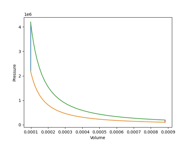
The various process were printed using plot from matplotlib.pyplot module. The x-axis was named as Volume and y-axis was names as Pressure. The final plot is displayed using show from matplotlib.pyplot module.

Results:

Thermal efficiency for given values: 58.476%

PV Plot of Otto Cycle:

Conclusions:

• Program ran successfully
• The Adiabatic Processes are Parabolic in Nature on the plot due to power Gamma
• The Isochoric Processes are straight lines due to constant volume