Solving 2nd Order ODEs & Simulation Motion of a Pendulum in Python

Aim:

To write a python program that will simulate the transient motion of a pendulum with given parameters.

Governing Equations & Theory:

The following is the second order Ordinary Differential Equation (ODE) given, which represents a simple pendulum under damped oscillatory motion.

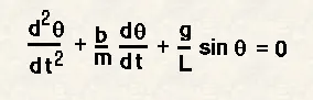  Where,

b = damping coefficient (no units) = 0.05

m = mass of the ball (kg) = 1

g = acceleration due to gravity (m/s^s) = 9.81

l = length of pendulum (m) = 1

As stated, above is an Ordinary Differential Equation which represents the motion of a simple pendulum. Upon solving this equation, we can derive a function which tells us the position of the pendulum at a given point in time.

We can solve it by using the known variables in the equation.

This particular simple pendulum takes damping into account, which is a factor in real life, this damping factor reduces the amplitude of the pendulum over time. Damping can occur due to a number of factors like air resistance, friction, etc., which are all considered into the final value of the damping coefficient.

 

Objectives:

• To plot position of pendulum as function of time.
• To create an animation of the motion of the pendulum.

Body of the Contents:

Python was the language used to code the following programs.

Program:

 # 1st Part: Solving ODE representing motion of simple pendulum
 # 2nd Part: Simulating motion of Pendulum with Animation

"""
First Part
"""
#Solving ODE
#importing required modules
import numpy as np 
from scipy.integrate import odeint
import matplotlib.pyplot as plt
import math

#Defining a function that returns dz/dt from given ODE
def model(theta,t,b,g,l,m):
	theta1 = theta[0]
	theta2 = theta[1]
	dtheta1_dt = theta2
	dtheta2_dt = -(b/m)*theta2 -(g/l)*math.sin(theta1)
	dtheta_dt = [dtheta1_dt, dtheta2_dt]
	return dtheta_dt

#given paramters to solve ODE for motion of simple pendulum
b = 0.05	#no units
g = 9.81	#m/s^2
l = 1		#metre    
m = 1		#kg

# Initial Condition
theta_0 = [math.pi/2,0]

# Time Points 
t = np.linspace(0,20,150) #we have taken 150 points in time until 20s

# ODE solve
theta = odeint(model,theta_0,t, args = (b,g,l,m))

#plotting the results
plt.plot(t,theta[:,0],'b-', label=r'$frac{dtheta_1}{dt}=theta2$')
plt.plot(t,theta[:,1],'r--', label=r'$frac{dtheta2}{dt}=-frac{b}{m}theta_2-|frac{g}{L}sintheta_1$')
plt.ylabel("Plot")
plt.xlabel("Time")
plt.legend(loc = 'best')
plt.show()

"""
Second Part
"""
#The Animation 
 
count = 1   #counter variable
x0 = 0		#fixed end coordinate
y0 = 0		#fixed end coordinate

for i in range (len(t)):
	#coordinates of Pendulum Bob
	x1 = x0 + l*math.sin(theta[i,0])
	y1 = y0 - l*math.cos(theta[i,0])

	filename = 'PendulumPos%05d.png' %count #to make sure there is no conflice in filenames
	

	plt.figure()	# to ensure new figure for each position
	plt.plot([-1,1],[0,0],"black", linewidth =3)	#Attachment line

	plt.plot([x0,x1],[y0,y1],"blue")	#String attaching bob

	plt.plot(x1,y1,'o', markersize= 13)		#Bob

	plt.xlim([-1,1])
	plt.ylim([-2,1.5])

	plt.savefig(filename)
	count = count + 1

All the required modules like numpy, math, matplotlib.pyplot, odeint (from scipy.integrate) were imported at the start. The code was split into 2 parts; the solving, plotting of ODE and the Animation of Pendulum.

A function was defined to give the value of  which is necessary to use odeint module to solve the equation. All the input parameters which would be needed later on were given as arguments to facilitate the same.

The given parameters for the pendulum were intialised. And linspace from numpy module was used to generate 150 points of time from 0 to 20s, each of which being a data point at which the position would be calculated for both plotting and the simulation video.

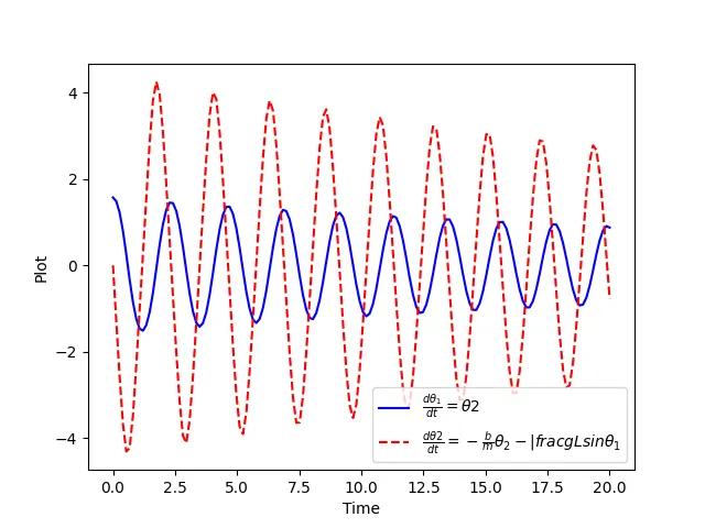
Using odeint, the equation was solved and the solution i.e., the required coordinates were stored into an array. The data was then plotted as shown later on with a legend.

The Animation required multiple images, each at a point in time (defined earlier) and the corresponding coordinates of the pendulum. This was done by assuming the origin to be the fixed end of the pendulum and simple trigonometric functions defining the (x,y) coordinates using the value of angle  at each point obtained by solving the ODE. After adding some aesthetics, and adding limiters on the axes to maintain uniformity the files were saved with unique and sequential names.

Results:

1. The link for simulation: https://youtu.be/Fh1kt1L7Jvo
2. The plot:

Conclusions:

• Program ran successfully
• The damping coefficient plays an important role in the amplitude
• The required plot was obtained