Curve Fitting using Python

Aim:

To write a python program that performs curve fitting.

Objectives:

1. What does popt and pcov mean?
2. What does np.array(temperature) do?
3. What does the * in *popt mean?
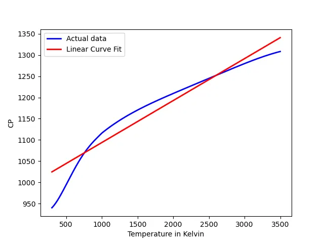
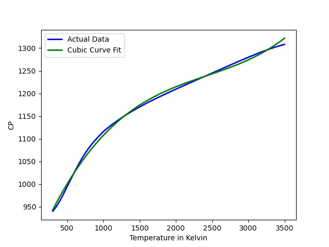
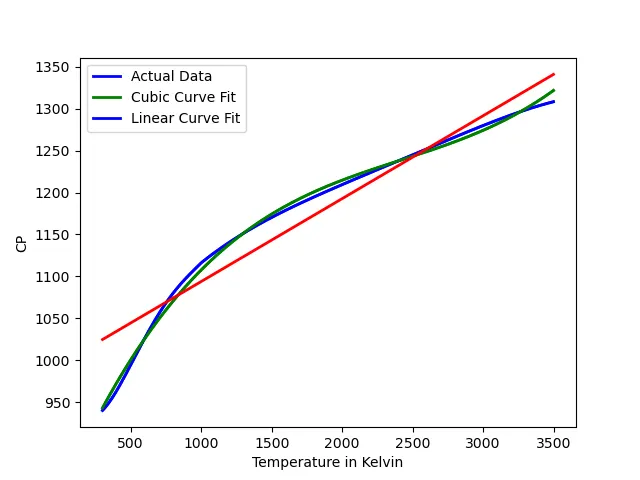
4. Write code to fit a linear and cubic polynomial for the Cp data. Explain if your results are good or bad. 
5. What needs to be done in order to make the curve fit perfect?
6. Show empirically as to how well your curve has been fit.

Body of the Contents:

Answers to questions:

1. What does popt and pcov mean?

Popt is an array which contains the parameters used for ‘fit’, which are found by calculating curve fitting. Pcov is another array to which is used to store ‘covariance’ values.

2. What does np.array(temperature) do?

It used to pass the temperatures as a numpy array to the function

3. What does the * in *popt mean?

‘*’ in an any array, in this case popt is used to refer to and select the values in it.

5.  What needs to be done in order to make the curve fit perfect?

As it can be concluded from the results in the end, the higher the order of the polynomial, the better the fit.

Program:

Question 4:

import numpy as np
from scipy.optimize import curve_fit
import matplotlib.pyplot as plt

def f1(x, a, b):
    return a*x + b

def f2(x, a, b, c, d):
    return a*pow(x, 3) + b*pow(x, 2) + c*x + d

def read_file():
    temp =[]
    cp = []
    for line in open("data", "r"):
        values = line.split(",")
        temp.append(float(values[0]))
        cp.append(float(values[1]))
    
    return [temp, cp]

temp, cp = read_file()
pop_t, pcov = curve_fit(f1, temp, cp)
pop_t2, pcov2 = curve_fit(f2, temp, cp)
fit_cp = f1(np.array(temp), *pop_t)
fit_cp_1 = f2(np.array(temp), *pop_t2)

#Curve Plotting

#Linear Curve fit
plt.plot(temp, cp, color= "blue", linewidth = 2)
plt.plot(temp, fit_cp, color= "red", linewidth = 2)
plt.xlabel("Temperature in Kelvin")
plt.ylabel("CP")
plt.legend(["Actual data", "Linear Curve Fit"])
plt.savefig("Linear_Fit")
plt.show()
plt.clf()

#Cubic Curve Fit
plt.xlabel("Temperature in Kelvin")
plt.ylabel("CP")
plt.plot(temp, cp, color= "blue", linewidth = 2)
plt.plot(temp, fit_cp_1, color ="green", linewidth = 2)
plt.legend(["Actual Data", "Cubic Curve Fit"])
plt.savefig("Cubic_Fit")
plt.show()

#Both Curves fit
plt.plot(temp, cp, color= "blue", linewidth = 2)
plt.plot(temp, fit_cp_1, color ="green", linewidth = 2)
plt.plot(temp, fit_cp, color= "red", linewidth = 2)
plt.legend(["Actual Data", "Cubic Curve Fit", "Linear Curve Fit"])
plt.savefig("Curves_Both")
plt.show()


#constants

number_pts = np.size(cp)
total = np.sum(cp)
mean = total/number_pts

#Linear Curve
linear_sse = 0
liner_ssr = 0

for i in range(number_pts):
    lerr = abs((np.sum((cp[i] - fit_cp[i]))))
    linear_sse = linear_sse + pow(lerr,2)
    liner_ssr = liner_ssr + np.sum(pow((fit_cp[i] - mean),2))

 
linear_sst = linear_sse + liner_ssr
linear_rmse = pow((linear_sse/number_pts),0.5)
linear_sqr = liner_ssr/linear_sst

print("R Square value for the Linear Curve Fit is:",linear_sqr)


#Cubic Curve
cubic_sse = 0
cubic_ssr = 0

for j in range(number_pts):
    cubic_err = abs(np.sum((cp[i] - fit_cp_1[i])))
    
    cubic_sse = cubic_sse+(pow(cubic_err,2))
    cubic_ssr = cubic_ssr+np.sum(pow((fit_cp_1[i] - mean),2))

 
cubic_sst = cubic_sse + cubic_ssr
cubic_rmse = pow((cubic_sse/number_pts),0.5)
cubic_rsq= cubic_ssr/cubic_sst


print("R Square value for the Cubic Curve Fit:",cubic_rsq)

Python was the language used to code the above program.

All the required modules like numpy, math, matplotlib.pyplot, curve_fit (from scipy.integrate) were imported at the start. The functions for both the linear and cubic polynomials are defined. Another function to read the given ‘data’ file is defined, since the file is separated by commas, comma is used a delimiter to split the file to store the output into respective arrays.

Since the values are now with us, curve_fit is used and they are used in the functions to get the initial curve.

The Linear curve is plotted with respective legends and named axes. This plot comparison is saved with the respective name.

The Cubic curve is then plotted with respective legends and named axes. This plot comparison is saved with the respective name.

Another curve with both the Cubic and Linear curves are plotted, saved and showed.

The R. Square value of the of both the curves are found and printed using the required formulae.

Results:

• The output as an image:

6th Question:

• The Linear Curve Plot:

• The Cubic Curve Plot:

• The Plot with both Curves:

 

Conclusions:

• Program ran successfully
• Higher order gives a better fit