Week 2 Air standard Cycle

Aim:

To plot PV diagram of otto cycle of an engine for the given set of dimension

Formulae Required

Swept volume(`V_s`) = `pi/4`*`B^2`*S

clearance volume(`V_c`) = `V_S/(C_r-1)`

Relation between volume and crank angle is

`V/V_C = 1 + (C_r-1)/2[R + 1- costheta-(R^2-sin^2theta)^(1/2)]`

Here the terms in the above equations are

B = bore of the engine

S = length of stroke

`theta` = crank angle

`C_r =`compression ratio

`V_c`= clearance volume

R = `2*(l/s)`

Objective

otto cycle is also can be considered as petrol engine cycle in we can observe two isochoric cycles and two adibatic cycles.

Procedure

The progamming required to plot the otto cycle curve is given below

import math
import matplotlib.pyplot as plt
import numpy as np
#function for generating volumes for different crank angles
def engine_kinematics(bore,stroke,con_rod,CR,start_crank,end_crank):
    bore=0.10
    stroke=0.1
    con_rod=0.15
    CR=12
    a=stroke/2
    R=con_rod/a
    V_s=math.pi/4*pow(bore,2)*stroke
    V_c=V_s/(CR-1)
#crank angles are taken as dtheta
    sc=math.radians(start_crank)
    ec=math.radians(end_crank)
    num_values=50
    dtheta=(ec-sc)/(num_values-1)
    v=[]
    for i in range(0,num_values):
        theta=sc+i*dtheta
        term1=0.5*(CR-1)
        term2=R+1-math.cos(theta)
        term3=pow(R,2)-pow(math.sin(theta),2)
        term4=pow(term3,0.5)
        v.append((1+term1*(term2-term4))*V_c)
    return(v)

#temparature,pressure
p1=101325
t1=500
gamma=1.4
t3=2300
#dimensions of engine
bore=0.1
stroke=0.1
con_rod=0.15
CR=12
#sweptvolume
v_s=(math.pi/4)*pow(bore,2)*stroke
v_c=v_s/(CR-1)
v1=v_c+v_s
#state point2
v2=v_c
p2=p1*pow(v1,gamma)/pow(v2,gamma)
#calculate t2
lhs=(p1*v1)/t1
t2=(p2*v2)/lhs
v_compression=engine_kinematics(bore,stroke,con_rod,CR,180,0)
constant=p1*pow(v1,gamma)
p_compression=[]
for v in v_compression:
    p_compression.append(constant/pow(v,gamma))
#state point3
v3=v2
rhs=(p2*v2)/t2
p3=rhs*t3/v3
v_expansion=engine_kinematics(bore,stroke,con_rod,CR,0,180)
constant=p3*pow(v3,gamma)
p_expansion=[]
for v in v_expansion:
    p_expansion.append(constant/pow(v,gamma))
#state point4
v4=v1
p4=p3*pow(v3,gamma)/pow(v4,gamma)
t4=p4*v4/lhs
#plotting otto cycle
plt.plot([v2,v3],[p2,p3],label='heat addition')
plt.plot(v_compression,p_compression,label='compression')
plt.plot(v_expansion,p_expansion,label='expansion')
plt.plot([v4,v1],[p4,p1],label='heat rejected')
plt.legend(['heat addition','compression','expansion','heat rejection'],loc="upper right")
plt.savefig("ottocycle.png")
plt.show()
#thermal efficiency
Th_ef=(1-1/(pow(CR,(gamma-1))))*100
print("thermalefficiency is:")
print(Th_ef)

Here we use function for calling the value of bore ,stroke,connecting rod length,compression ratio,starting crank angle and end crank angle for determing the values of respective volumes and pressures in order to plot the curves.If donot consider the crank angle then the curve would be of staright lines which is not correct but when we include crank angles to find respective parameters we could get a nice smooth cureve of otto cycle. From this we can able to find thermal efficiency of otto cycle by using a simple formula.In this way we can the thermal efficiency and we can get a plot of smooth curve.

PV diagram of otto cycle obtained from above values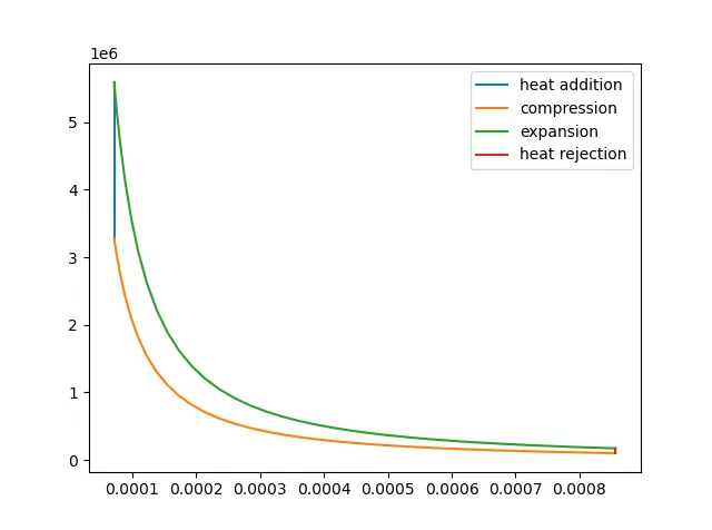

The thermal efficiency obtained by using the assigned values is 62.9892

Conclusion

The pv diagram of otto cycle is plotted by using the concepts of forward dynamics and also obtained the value of thermal efficiency.