Week 3 - Solving second order ODEs

Aim

To solve the damped oscillation equation with following inputs and represent the plots of pendulum into animation.

`(d^2theta)/dt^2+b/m(d theta)/(dt )+g/Lsintheta=0`

by taking

b = 0.005

g = 9.81(m/`s^2`)

l = 1(m)

m = 0.1(kg)

Theory

The equation of damped oscillations is 2nd order ordinary differential equation with damping constant as b.The reason why it is 2nd order ODE is the equation has one double derivative.Here we can see there are two main parameters involved in this equation. `theta`is the displacement and t is the time. so the plot is represented between these parameters.To solve this ODE in python we need to install scipy module.From scipy module we import odeint to solve the integration.

Procedure

Here we assume some terms for simplification

`theta = theta_1`

`(d theta_1)/(dt) = theta_2`

we moved to this step for easy simplification of ode

The python code for the simplification of this ode with the above inputs

#solving 2nd order of ODE of damped oscillations of simple pendulum
import numpy as np
import matplotlib.pyplot as plt 
from scipy.integrate   import odeint
import math

#function that returns dz/dt
def model(theta,t,b,g,l,m):

	theta1 = theta[0]
	theta2 = theta[1]

	dtheta1_dt = theta2
	dtheta2_dt = (b/m)*theta2 - (g/l)*math.sin(theta1)
	dtheta_dt = [dtheta1_dt,dtheta2_dt]
	return dtheta_dt
#inputs	

b = 0.005
g = 9.81
l = 1
m = 0.1
# initial condition

theta0 = [math.pi/2,0]

#timepoints
t = np.linspace(0,10,150)

#solve ode
theta = odeint(model,theta0,t,args = (b,g,l,m))

#plot results
plt.plot(t,theta[:,0],'b-',label=r'$\frac{d\theta_1}{dt}=\theta2$')
plt.plot(t,theta[:,1],'r--',label=r'$\frac{d\theta_2}{dt}=-\frac{b}{ m}\theta_2-\frac{g} {L}sin\theta_1$')
plt.ylabel('plot')
plt.xlabel('time')
plt.legend(loc='best')


theta_x1 = 0
theta_x2 = 3
t_x = theta[:,0]
#plotting graph
for i in range(0,100):
	plt.plot([0,1],[theta_x1,t_x[i]],marker = 'o')
	plt.xlim([-5,5])
	plt.ylim([-5,5])
	plt.figure()
	plt.savefig('forward.png')
	plt.show()
	

In the code we installed scipy module for solving ode

here we defined a function called module in which it has displacement(`theta`),time , damping coefficient,length,mass,acceleration due to gravity

Here we sovle this by converting the ode in to simple matrix and then we solve the matrix.

Here we have the `theta` range of pi/2 to 0 degrees

so we get a plot against displace ment and time in the below manner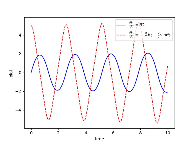

as we splitted the ODEs to form simple matrix, the first ode graph starts with displacement > 0 and 2nd ODE starts with zero displacement. If we observe the graph as the time increases both of the ODEs displacement gets decreased. In this the dampers work.These ODEs play major role in automobile industries which helps in designing dampers of vehicles.

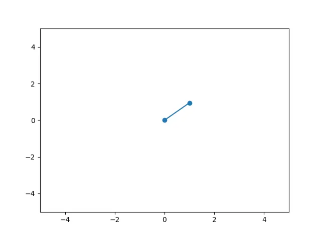
The final part of the code is to create animation of plots of pendulum for that the logic is to create each plot for each value of time so that as the time changes we some 100 plots (as my range is 100) and we animate them to form a gif. The below link is the animation

the sample of the animation is

Conclusion

As the time increases the displacement gets decreases in the damped oscillations.These concepts play an important role in designing of dampers.