Week 12 - Validation studies of Symmetry BC vs Wedge BC in OpenFOAM vs Analytical H.P equation
Objective:
- To simulate an axis-symmetric laminar flow through the constant cross-sectional of the pipe by applying the symmetry boundary condition.
- To simulating for the mentioned angles i.e for 10, 25, 45 degrees using both symmetry and wedge boundary conditions and validate them with HP equations.
Expected Results:
- Validate Hydro-dynamic length with the numerical result
- Validate the fully developed flow velocity profile with its analytical profile
- Validate maximum velocity and pressured drop for fully developed flow
- Post-process Shear stress and validate wall shear stress for fully developed flow
- Highlight the differences in both boundary conditions in terms of their usage and application
Hagen-Poiseuille's law:
In non-ideal fluid dynamics, the Hagen–Poiseuille equation, also known as the Hagen–Poiseuille law, is a physical law that gives the pressure drop in an incompressible and Newtonian fluid in laminar flow flowing through a long cylindrical pipe of constant cross-section. The pressure drop is given by:
ΔP = 32μLV/D2
where,
ΔP. is the pressure drop.
μ is the dynamic viscosity.
L is the length of the pipe.
V is the velocity.
At the entrance, the flow is said to be in hydrodynamic entrance region where the velocity profile gradually takes the shape of a parabola from a straight line. As soon as the parabolic velocity profile becomes steady the flow is said to be in its fully developed state. Normally Hagen Poiseuille's Equation is applicable for fully developed flow which helps us to calculate the pressure loss.
For a circular pipe, we can calculate the average and maximum velocity, maximum shear stress and pressure loss analytically which are as follows.
Assumptions made:
Geometry: Axisymmetric.
Reynolds number: 2100.
Working fluid: Water.
Diameter of the pipe: 0.02 m.
Dynamic viscosity(μ)=0.89x10^-3 Pas
Kinematic viscosity(ν)=0.8927x10^-6 m^2/s
theta=10, 25, 45
EQUATIONS USED:
Average velocity
Vavg = μRe/ρDh m/s
Maximum velocity
Vmax=2 * Vavg m/s
τmax=2μV/rh
Hagen Poiseuille's Equation (Pressure drop):
ΔP =Ploss=32μ(L−Le)Vavg/D2ℎ
Here
Vavg = Average velocity
Vmax = maximum velocity
τmax = maximum shear stress
μ = dynamic viscosity
Dℎ = hydraulic diameter of the pipe
rℎ= hydraulic radius of the pipe
Ploss = pressure loss
Le = Entrance Length = 0.06 Re Dℎ (For laminar flow through a circular pipe)
kinematic pressure drop=ΔP /ρ
Problem definition:
Here we are considering a circular pipe of 20 mm diameter and 3.02 m length through which the flowing fluid is water with density of 997 kg/m^3 and dynamic viscosity of 0.00089 Pa.s
As per the calculations, the keep the flow laminar the average velocity of the flow is taken to be 0.1875 m/s and thus the Reynolds's Number, Re = 2100. For a circular pipe the flow becomes turbulent after when Reynolds's number becomes greater than 4000 and in between 2300-4000 the flow remains in the transition state.
PROCEDURE:
- We will start with copying the cavity file from the tutorial to the FOAM_RUN folder.
- In the run folder only we are going to simulate and whatever we want to do the changes in the blockMeshDict file and pressure and velocity files and controlDict files we will be doing here.
- Creating the block in the OpenFoam here we are creating the wedge after making the required changes in the blockMeshDict file to check the geometry run the blockMesh command.
- After creating the wedge assign the boundary conditions, and also sitting the simulation end time and time-step in such a way that the courant number should be less than 0.5 and also in the transportProperties enter the kinematic viscosity.
- Run the simulation using the icoFoam solver after calculating the time needed for the fluid to travel from inlet to outlet
- After the simulation, use paraFoam to view the flow inside the wedge and use plot over line command to plot the velocity and shear stress changes at a point after the hydrodynamical entry region so that we analyse the fully developed region of the fluid.
- Use Matlab to parse the blockMeshDict so that the same file can be used for any wedge values.
Solver:
To solve the incompressible problem and the above mentioned equation we have selected the icoFOAM solver of openFOAM.
Code:
Matlab programme for automatically generate blockMeshDict file for a wedge boundary conditions
<![endif]-->
<![endif]-->
<![endif]-->
<![endif]-->
For wedge boundary conditions.
For the wedge angle 10 degrees the blockMeshDict file.
OpenFOAM Files:
1. System Folder:
a. blockMeshDict:
 /*---------------------------------*- C++ -*-------------------------------------------------*\
 | ==========      |                                                                           |
 | \\        /  F ield        | OpenFOAM: The Open Source CFD Toolbox                          |
 |  \\      /   O peration    | Version:  9                                                    |
 |   \\    /    A nd          | Web:      www.OpenFOAM.org                                     |
 |    \\  /     M anipulation |                                                                |
  \*------------------------------------------------------------------------------------------*/
 FoamFile
{
     format         ascii;
     class          dictionary;
     object         blockMeshDict;
}
 // * * * * * * * * * * * * * * * * * * * * * * * * * * * * * * * * * * * * * * * * * * * * *  \\
convertToMeters 1;
vertices
(
(0.000000 0.000000 0.000000)
(0.000872 0.009962 0.000000)
(-0.000872 0.009962 0.000000)
(0.000000 0.000000 3.020000)
(0.000872 0.009962 3.020000)
(-0.000872 0.009962 3.020000)
);
blocks
(
hex (0 0 1 2 3 3 4 5) (1 40 500) simpleGrading (1 1 1)
);
edges
(
arc 1 2 (0.000000 0.010000 0.000000)
arc 4 5 (0.000000 0.010000 3.020000)
);
boundary
(
inflow
{
type patch;
faces
(
(0 0 2 1)
);
}
outflow
{
type patch;
faces
(
(3 4 5 3)
);
}
front
{
type wedge;
faces
(
(0 1 4 3)
);
}
back
{
type wedge;
faces
(
(3 5 2 0)
);
}
wall
{
type wall;
faces
(
(4 1 2 5)
);
}
axis
{
type empty;
faces
(
(0 3 3 0)
);
}
);
mergePatchPairs
(
);
// ************************************************************************************************************************************************** //
b. controlDict
/*--------------------------------*- C++ -*----------------------------------*\
  =========                 |
  \\      /  F ield         | OpenFOAM: The Open Source CFD Toolbox
   \\    /   O peration     | Website:  https://openfoam.org
    \\  /    A nd           | Version:  9
     \\/     M anipulation  |
\*---------------------------------------------------------------------------*/
FoamFile
{
    format      ascii;
    class       dictionary;
    location    "system";
    object      controlDict;
}
// * * * * * * * * * * * * * * * * * * * * * * * * * * * * * * * * * * * * * //

application     icoFoam;

startFrom       latestTime;

startTime       0;

stopAt          endTime;

endTime         10;

deltaT          0.01;

writeControl    timeStep;

writeInterval   20;

purgeWrite      0;

writeFormat     ascii;

writePrecision  6;

writeCompression off;

timeFormat      general;

timePrecision   6;

runTimeModifiable true;


// ************************************************************************* //
2. constant Folder:
a. transportProperties
/*--------------------------------*- C++ -*----------------------------------*\
  =========                 |
  \\      /  F ield         | OpenFOAM: The Open Source CFD Toolbox
   \\    /   O peration     | Website:  https://openfoam.org
    \\  /    A nd           | Version:  9
     \\/     M anipulation  |
\*---------------------------------------------------------------------------*/
FoamFile
{
    format      ascii;
    class       dictionary;
    location    "constant";
    object      transportProperties;
}
// * * * * * * * * * * * * * * * * * * * * * * * * * * * * * * * * * * * * * //

nu              [0 2 -1 0 0 0 0] 0.8927e-06;


// ************************************************************************* //
3. 0 Folder
a. U (velocity)
/*--------------------------------*- C++ -*----------------------------------*\
  =========                 |
  \\      /  F ield         | OpenFOAM: The Open Source CFD Toolbox
   \\    /   O peration     | Website:  https://openfoam.org
    \\  /    A nd           | Version:  9
     \\/     M anipulation  |
\*---------------------------------------------------------------------------*/
FoamFile
{
    format      ascii;
    class       volVectorField;
    object      U;
}
// * * * * * * * * * * * * * * * * * * * * * * * * * * * * * * * * * * * * * //

dimensions      [0 1 -1 0 0 0 0];

internalField   uniform (0 0 0);

boundaryField
{
    inflow
    {
        type            fixedValue;
        value           uniform (0 0 0.1875);
    }

    outflow
    {
        type            zeroGradient;
    }

    wall
    {
        type            noSlip;
    }

    front
    {
        type            wedge;
    }

    back
    {
        type            wedge;
    }

    axis
    {
        type            empty;
    }

}

// ************************************************************************* //
b. p (Pressure)
/*--------------------------------*- C++ -*----------------------------------*\
  =========                 |
  \\      /  F ield         | OpenFOAM: The Open Source CFD Toolbox
   \\    /   O peration     | Website:  https://openfoam.org
    \\  /    A nd           | Version:  9
     \\/     M anipulation  |
\*---------------------------------------------------------------------------*/
FoamFile
{
    format      ascii;
    class       volScalarField;
    object      p;
}
// * * * * * * * * * * * * * * * * * * * * * * * * * * * * * * * * * * * * * //

dimensions      [0 2 -2 0 0 0 0];

internalField   uniform 0;

boundaryField
{
    inflow
    {
        type  zeroGradient;
    }

    outflow
    {
        type            fixedValue;
        value           uniform 0;
    }

    wall
    {
        type          zeroGradient;
    }

   front
    {
        type            wedge;
    }

   back
    {
        type            wedge;
    }

   axis
    {
        type            empty;
    }
}

// ************************************************************************* //
Algorithm:
1. In the first step we have defined the geometry parameters and then passed the radius, length of pipe and wedge angle to the system() function which basically printed the blockMeshDict file.
2. We have set the file structure of the openFOAM for the icoFoam solver.
3. Afterwards we have typed the following keys on the xterm terminal to simulate the setup
blockMesh -> checkMesh -> icoFoam
4. Post-processing was accomplished using paraView.
Use solver icoFoam to solve problem.
icoFoam Transient solver for incompressible, laminar flow of Newtonian fluids
This will solve for timestep 30 with interval of 20 asper controlDict.
Results:
blockMesh
Velocity profile
Pressure profile
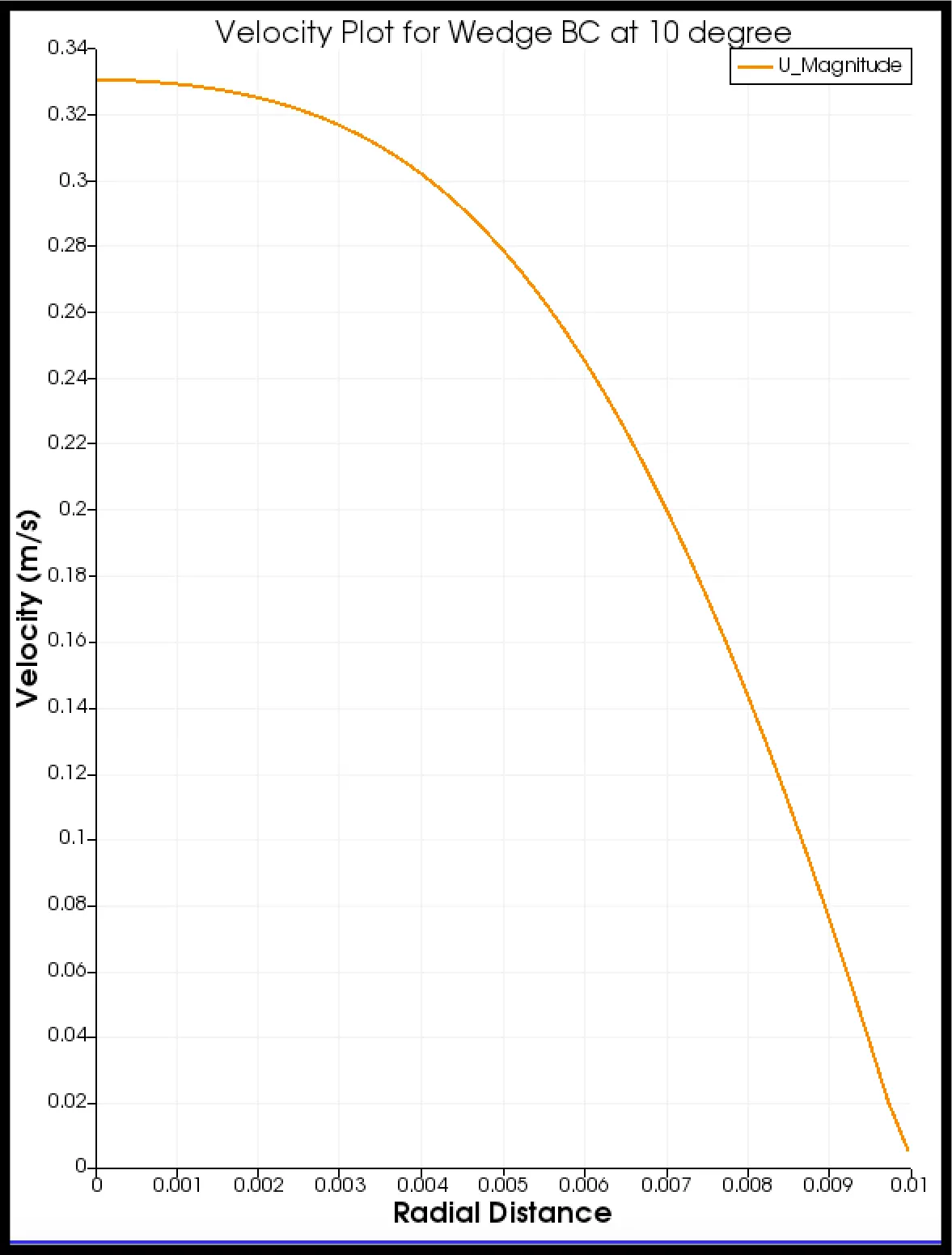
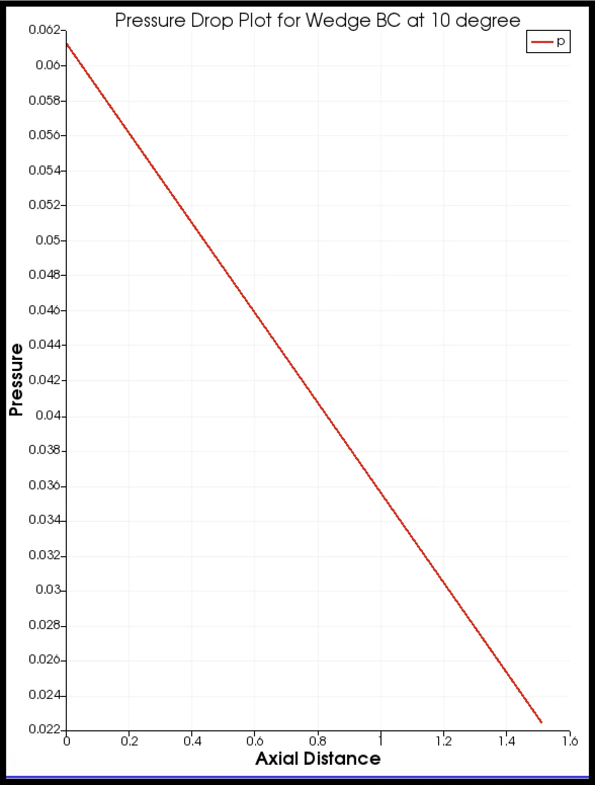
pressure =(0.061-0.022)=0.039
For wedge boundary conditions.
For the angle 25 degrees the blockMeshDict file.
 /*---------------------------------*- C++ -*-------------------------------------------------*\
 | ==========      |                                                                           |
 | \\        /  F ield        | OpenFOAM: The Open Source CFD Toolbox                          |
 |  \\      /   O peration    | Version:  9                                                    |
 |   \\    /    A nd          | Web:      www.OpenFOAM.org                                     |
 |    \\  /     M anipulation |                                                                |
  \*------------------------------------------------------------------------------------------*/
 FoamFile
{
     format         ascii;
     class          dictionary;
     object         blockMeshDict;
}
 // * * * * * * * * * * * * * * * * * * * * * * * * * * * * * * * * * * * * * * * * * * * * *  \\

convertToMeters 1;

vertices
(
      (0.000000 0.000000 0.000000)
      (0.002164 0.009763 0.000000)
      (-0.002164 0.009763 0.000000)
      (0.000000 0.000000 3.020000)
      (0.002164 0.009763 3.020000)
      (-0.002164 0.009763 3.020000)
);

blocks
(
      hex (0 0 1 2 3 3 4 5) (1 40 500) simpleGrading (1 1 1)
);

edges
(
      arc 1 2 (0.000000 0.010000 0.000000)
      arc 4 5 (0.000000 0.010000 3.020000)
);

boundary
(
      inflow
      {
           type patch;
           faces
           (
                (0 0 2 1)
           );
      }
      outflow
      {
           type patch;
           faces
           (
                (3 4 5 3)
           );
      }
      front
      {
           type wedge;
           faces
           (
                (0 1 4 3)
           );
      }
      back
      {
           type wedge;
           faces
           (
                (3 5 2 0)
           );
      }
      wall
      {
           type wall;
           faces
           (
                 (4 1 2 5)
           );
      }
      axis
      {
           type empty;
           faces
           (
                 (0 3 3 0)
           );
      }
);

mergePatchPairs
(
);

// ************************************************************************************************************************************************** //
Results:
blockMesh
Velocity profile
Pressure profile
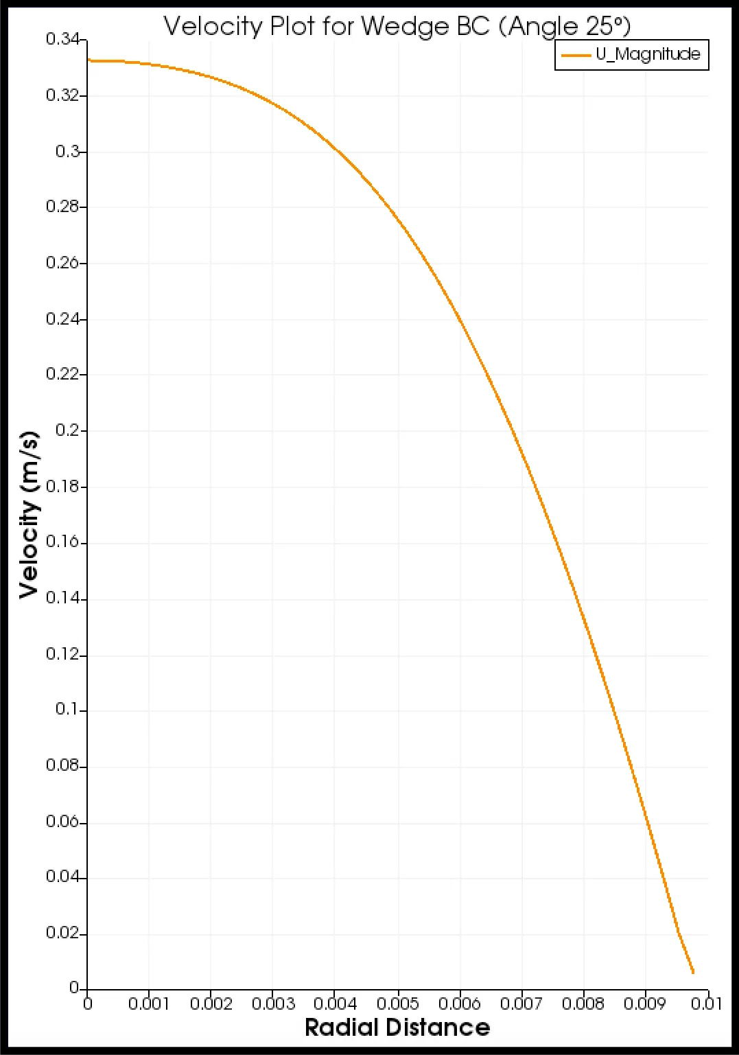
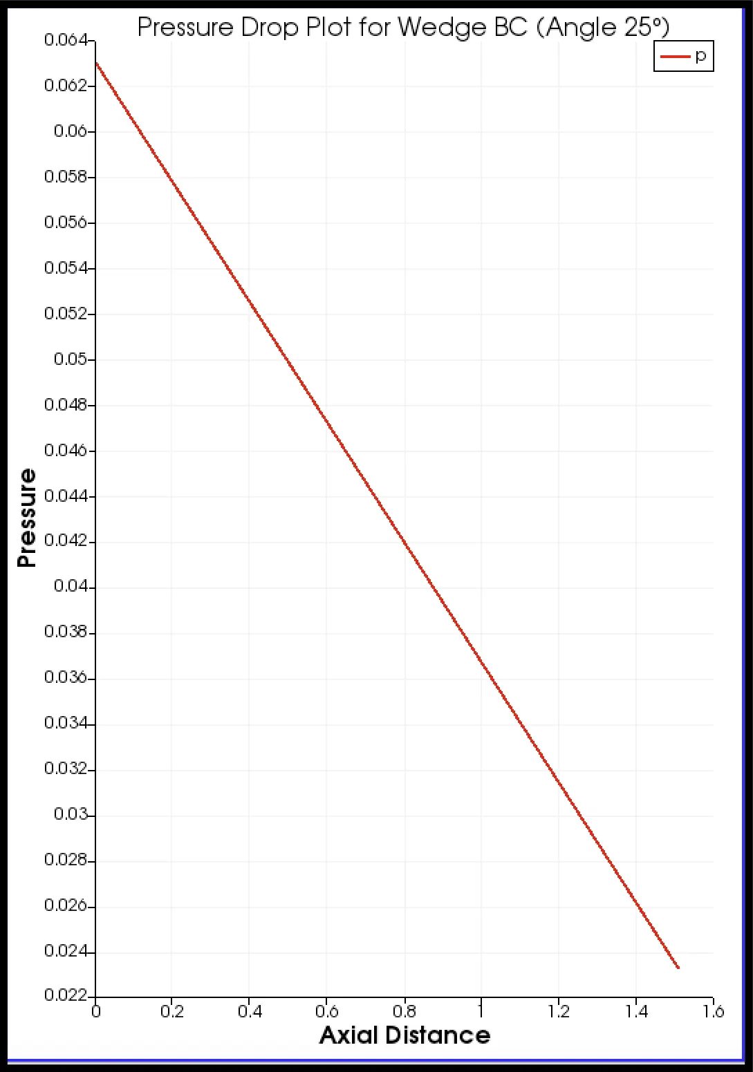
Pressure drop = (0.063-0.023)=0.04
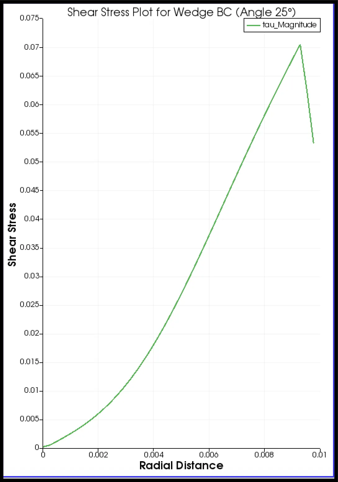
For wedge boundary conditions.
For the angle 45 degrees the blockMeshDict file.
 /*---------------------------------*- C++ -*-------------------------------------------------*\
 | ==========      |                                                                           |
 | \\        /  F ield        | OpenFOAM: The Open Source CFD Toolbox                          |
 |  \\      /   O peration    | Version:  9                                                    |
 |   \\    /    A nd          | Web:      www.OpenFOAM.org                                     |
 |    \\  /     M anipulation |                                                                |
  \*------------------------------------------------------------------------------------------*/
 FoamFile
{
     format         ascii;
     class          dictionary;
     object         blockMeshDict;
}
 // * * * * * * * * * * * * * * * * * * * * * * * * * * * * * * * * * * * * * * * * * * * * *  \\

convertToMeters 1;

vertices
(
      (0.000000 0.000000 0.000000)
      (0.003827 0.009239 0.000000)
      (-0.003827 0.009239 0.000000)
      (0.000000 0.000000 3.020000)
      (0.003827 0.009239 3.020000)
      (-0.003827 0.009239 3.020000)
);

blocks
(
      hex (0 0 1 2 3 3 4 5) (1 40 500) simpleGrading (1 1 1)
);

edges
(
      arc 1 2 (0.000000 0.010000 0.000000)
      arc 4 5 (0.000000 0.010000 3.020000)
);

boundary
(
      inflow
      {
           type patch;
           faces
           (
                (0 0 2 1)
           );
      }
      outflow
      {
           type patch;
           faces
           (
                (3 4 5 3)
           );
      }
      front
      {
           type wedge;
           faces
           (
                (0 1 4 3)
           );
      }
      back
      {
           type wedge;
           faces
           (
                (3 5 2 0)
           );
      }
      wall
      {
           type wall;
           faces
           (
                 (4 1 2 5)
           );
      }
      axis
      {
           type empty;
           faces
           (
                 (0 3 3 0)
           );
      }
);

mergePatchPairs
(
);

// ************************************************************************************************************************************************** //
Results:
blockMesh
Velocity profile
Pressure profile
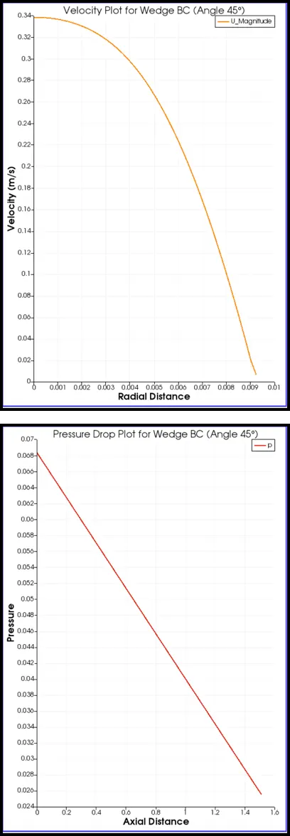
Pressure drop = (0.0683-0.0255)=0.0428
MATLAB CODE TO GENERATE blockMeshDict file for symmetry boundary condition.
clear all
close all
clc
% inputs
% assumptions made the fluid is assumed as water
Re=2100; % given Reynolds number
rho=997; �nsity of the water
D=0.02; % diameter of the pipe
r=D/2; % radius of the pipe
mu=0.89*10^-3; % dynamic viscosity of the water at 25 degree celsius
v=0.8927*10^-6; % kinematic viscosity of the water at 25 degree celsius
theta=input('Enter the value of the wedge angle = ')
Le=0.06*Re*D; % hydrodynamic length

L=Le+0.5;
% Analytical solutions
V_avg=(Re*mu)/(rho*D);  % average velocity
V_max=2*V_avg;   % maximum velocity
P_drop=(32*mu*(L-Le)*V_avg)/D^2;  % pressure drop
P_kinematic=(P_drop)/rho;  % kinematic pressure drop


 % String for header,
 h1 =' /*---------------------------------*- C++ -*-------------------------------------------------*\ ';
 h2 =' | ==========      |                                                                           |';
 h3 =' | \\        /  F ield        | OpenFOAM: The Open Source CFD Toolbox                          |';
 h4 =' |  \\      /   O peration    | Version:  9                                                    |';
 h5 =' |   \\    /    A nd          | Web:      www.OpenFOAM.org                                     |';
 h6 =' |    \\  /     M anipulation |                                                                |';
 h7 ='  \*------------------------------------------------------------------------------------------*/ ';
 h8 =' FoamFile';
 h9 ='{';

 h10 ='     format         ascii;';
 h11 ='     class          dictionary;';
 h12 ='     object         blockMeshDict;';
 h13 ='}';
 h14 =' // * * * * * * * * * * * * * * * * * * * * * * * * * * * * * * * * * * * * * * * * * * * * *  \\';

 conv ='convertToMeters 1;';

 sp1 = blanks(5);   %sp = space
 sp2 = blanks(10);
 sp3 = blanks(15);

 v_0 = [0 0 0];
 v_1 = [r*sind(theta/2) r*cosd(theta/2) 0];
 v_2 = [-r*sind(theta/2) r*cosd(theta/2) 0];
 v_3 = [0 0 L];
 v_4 = [r*sind(theta/2) r*cosd(theta/2) L];
 v_5 = [-r*sind(theta/2) r*cosd(theta/2) L];

 block ='hex (0 0 1 2 3 3 4 5) (1 40 500) simpleGrading (1 1 1)';
 edge1 ='arc 1 2';
 edge2 ='arc 4 5';

 e1 = [0 r 0];
 e2 = [0 r L];

 inlet = '(0 0 2 1)';
 outlet = '(3 4 5 3)';
 wedge1 = '(0 1 4 3)';
 wedge2 = '(3 5 2 0)';
 wall =' (4 1 2 5)';
 axis =' (0 3 3 0)';

 final = '// ************************************************************************************************************************************************** //';


 f1 = fopen('blockMeshDict_bc_symmetry','wt');

 fprintf(f1,'%s\n',h1);
 fprintf(f1,'%s\n',h2);
 fprintf(f1,'%s\n',h3);
 fprintf(f1,'%s\n',h4);
 fprintf(f1,'%s\n',h5);
 fprintf(f1,'%s\n',h6);
 fprintf(f1,'%s\n',h7);
 fprintf(f1,'%s\n',h8);
 fprintf(f1,'%s\n',h9);
 fprintf(f1,'%s\n',h10);
 fprintf(f1,'%s\n',h11);
 fprintf(f1,'%s\n',h12);
 fprintf(f1,'%s\n',h13);
 fprintf(f1,'%s\n',h14);

 fprintf(f1,'\n');

 fprintf(f1,'%s\n',conv);
 fprintf(f1,'\n');


 fprintf(f1,'%s\n','vertices');
 fprintf(f1,'%s\n','(');
 fprintf(f1,'%s (%f %f %f) \n',sp1,v_0(1),v_0(2),v_0(3));
 fprintf(f1,'%s (%f %f %f) \n',sp1,v_1(1),v_1(2),v_1(3));
 fprintf(f1,'%s (%f %f %f) \n',sp1,v_2(1),v_2(2),v_2(3));
 fprintf(f1,'%s (%f %f %f) \n',sp1,v_3(1),v_3(2),v_3(3));
 fprintf(f1,'%s (%f %f %f) \n',sp1,v_4(1),v_4(2),v_4(3));
 fprintf(f1,'%s (%f %f %f) \n',sp1,v_5(1),v_5(2),v_5(3));
 fprintf(f1,'%s \n',');');
 fprintf(f1,'\n');


 fprintf(f1,'%s\n','blocks');
 fprintf(f1,'%s\n','(');
 fprintf(f1,'%s %s \n',sp1,block);
 fprintf(f1,'%s \n',');');
 fprintf(f1,'\n');

  fprintf(f1,'%s \n','edges');
  fprintf(f1,'%s \n','(');
  fprintf(f1,'%s %s (%f %f %f) \n',sp1,edge1,e1(1),e1(2),e1(3));
  fprintf(f1,'%s %s (%f %f %f) \n',sp1,edge2,e2(1),e2(2),e2(3));
  fprintf(f1,'%s \n',');');
  fprintf(f1,'\n');

   fprintf(f1,'%s \n','boundary');
   fprintf(f1,'%s \n','(');

  fprintf(f1,'%s %s \n',sp1,'inflow');
  fprintf(f1,'%s %s \n',sp1,'{');
  fprintf(f1,'%s %s \n',sp2,'type patch;');
  fprintf(f1,'%s %s \n',sp2,'faces');
  fprintf(f1,'%s %s \n',sp2,'(');
  fprintf(f1,'%s %s \n',sp3,inlet);
  fprintf(f1,'%s %s \n',sp2,');');
  fprintf(f1,'%s %s \n',sp1,'}');

   fprintf(f1,'%s %s \n',sp1,'outflow');
  fprintf(f1,'%s %s \n',sp1,'{');
  fprintf(f1,'%s %s \n',sp2,'type patch;');
  fprintf(f1,'%s %s \n',sp2,'faces');
  fprintf(f1,'%s %s \n',sp2,'(');
  fprintf(f1,'%s %s \n',sp3,outlet);
  fprintf(f1,'%s %s \n',sp2,');');
  fprintf(f1,'%s %s \n',sp1,'}');

   fprintf(f1,'%s %s \n',sp1,'front');
  fprintf(f1,'%s %s \n',sp1,'{');
  fprintf(f1,'%s %s \n',sp2,'type symmetry;');
  fprintf(f1,'%s %s \n',sp2,'faces');
  fprintf(f1,'%s %s \n',sp2,'(');
  fprintf(f1,'%s %s \n',sp3,wedge1);
  fprintf(f1,'%s %s \n',sp2,');');
  fprintf(f1,'%s %s \n',sp1,'}');

   fprintf(f1,'%s %s \n',sp1,'back');
  fprintf(f1,'%s %s \n',sp1,'{');
  fprintf(f1,'%s %s \n',sp2,'type symmetry;');
  fprintf(f1,'%s %s \n',sp2,'faces');
  fprintf(f1,'%s %s \n',sp2,'(');
  fprintf(f1,'%s %s \n',sp3,wedge2);
  fprintf(f1,'%s %s \n',sp2,');');
  fprintf(f1,'%s %s \n',sp1,'}');

   fprintf(f1,'%s %s \n',sp1,'wall');
  fprintf(f1,'%s %s \n',sp1,'{');
  fprintf(f1,'%s %s \n',sp2,'type wall;');
  fprintf(f1,'%s %s \n',sp2,'faces');
  fprintf(f1,'%s %s \n',sp2,'(');
  fprintf(f1,'%s %s \n',sp3,wall);
  fprintf(f1,'%s %s \n',sp2,');');
  fprintf(f1,'%s %s \n',sp1,'}');

   fprintf(f1,'%s %s \n',sp1,'axis');
  fprintf(f1,'%s %s \n',sp1,'{');
  fprintf(f1,'%s %s \n',sp2,'type empty;');
  fprintf(f1,'%s %s \n',sp2,'faces');
  fprintf(f1,'%s %s \n',sp2,'(');
  fprintf(f1,'%s %s \n',sp3,axis);
  fprintf(f1,'%s %s \n',sp2,');');
  fprintf(f1,'%s %s \n',sp1,'}');

  fprintf(f1,'%s \n',');');
  fprintf(f1,'\n');

  fprintf(f1,'%s \n','mergePatchPairs');
  fprintf(f1,'%s \n','(');
  fprintf(f1,'%s \n',');');
  fprintf(f1,'\n');
  fprintf(f1,'%s \n',final);

  fclose(f1);
For symmetry boundary conditions
For angle 10 degrees the blockMeshDict file
OpenFOAM Files:
1. System Folder:
a. blockMeshDict:
 /*---------------------------------*- C++ -*-------------------------------------------------*\
 | ==========      |                                                                           |
 | \\        /  F ield        | OpenFOAM: The Open Source CFD Toolbox                          |
 |  \\      /   O peration    | Version:  9                                                    |
 |   \\    /    A nd          | Web:      www.OpenFOAM.org                                     |
 |    \\  /     M anipulation |                                                                |
  \*------------------------------------------------------------------------------------------*/
 FoamFile
{
     format         ascii;
     class          dictionary;
     object         blockMeshDict;
}
 // * * * * * * * * * * * * * * * * * * * * * * * * * * * * * * * * * * * * * * * * * * * * *  \\

convertToMeters 1;

vertices
(
      (0.000000 0.000000 0.000000)
      (0.000872 0.009962 0.000000)
      (-0.000872 0.009962 0.000000)
      (0.000000 0.000000 3.020000)
      (0.000872 0.009962 3.020000)
      (-0.000872 0.009962 3.020000)
);

blocks
(
      hex (0 0 1 2 3 3 4 5) (1 40 500) simpleGrading (1 1 1)
);

edges
(
      arc 1 2 (0.000000 0.010000 0.000000)
      arc 4 5 (0.000000 0.010000 3.020000)
);

boundary
(
      inflow
      {
           type patch;
           faces
           (
                (0 0 2 1)
           );
      }
      outflow
      {
           type patch;
           faces
           (
                (3 4 5 3)
           );
      }
      front
      {
           type symmetry;
           faces
           (
                (0 1 4 3)
           );
      }
      back
      {
           type symmetry;
           faces
           (
                (3 5 2 0)
           );
      }
      wall
      {
           type wall;
           faces
           (
                 (4 1 2 5)
           );
      }
      axis
      {
           type empty;
           faces
           (
                 (0 3 3 0)
           );
      }
);

mergePatchPairs
(
);

// ************************************************************************************************************************************************** //
b. controlDict
/*--------------------------------*- C++ -*----------------------------------*\
  =========                 |
  \\      /  F ield         | OpenFOAM: The Open Source CFD Toolbox
   \\    /   O peration     | Website:  https://openfoam.org
    \\  /    A nd           | Version:  9
     \\/     M anipulation  |
\*---------------------------------------------------------------------------*/
FoamFile
{
    format      ascii;
    class       dictionary;
    location    "system";
    object      controlDict;
}
// * * * * * * * * * * * * * * * * * * * * * * * * * * * * * * * * * * * * * //

application     icoFoam;

startFrom       startTime;

startTime       0;

stopAt          endTime;

endTime         10;

deltaT          0.01;

writeControl    timeStep;

writeInterval   20;

purgeWrite      0;

writeFormat     ascii;

writePrecision  6;

writeCompression off;

timeFormat      general;

timePrecision   6;

runTimeModifiable true;


// ************************************************************************* //
2. constant Folder:
a. transportProperties
/*--------------------------------*- C++ -*----------------------------------*\
  =========                 |
  \\      /  F ield         | OpenFOAM: The Open Source CFD Toolbox
   \\    /   O peration     | Website:  https://openfoam.org
    \\  /    A nd           | Version:  9
     \\/     M anipulation  |
\*---------------------------------------------------------------------------*/
FoamFile
{
    format      ascii;
    class       dictionary;
    location    "constant";
    object      transportProperties;
}
// * * * * * * * * * * * * * * * * * * * * * * * * * * * * * * * * * * * * * //

nu              [0 2 -1 0 0 0 0] 0.8927e-06;


// ************************************************************************* //
3. 0 Folder
a. U (velocity)
/*--------------------------------*- C++ -*----------------------------------*\
  =========                 |
  \\      /  F ield         | OpenFOAM: The Open Source CFD Toolbox
   \\    /   O peration     | Website:  https://openfoam.org
    \\  /    A nd           | Version:  9
     \\/     M anipulation  |
\*---------------------------------------------------------------------------*/
FoamFile
{
    format      ascii;
    class       volVectorField;
    object      U;
}
// * * * * * * * * * * * * * * * * * * * * * * * * * * * * * * * * * * * * * //

dimensions      [0 1 -1 0 0 0 0];

internalField   uniform (0 0 0);

boundaryField
{
    inflow
    {
        type            fixedValue;
        value           uniform (0 0 0.1875);
    }

    outflow
    {
        type            zeroGradient;
    }

    wall
    {
        type            noSlip;
    }

    front
    {
        type            symmetry;
    }

    back
    {
        type            symmetry;
    }

    axis
    {
        type            empty;
    }

}

// ************************************************************************* //
b. p (Pressure)
/*--------------------------------*- C++ -*----------------------------------*\
  =========                 |
  \\      /  F ield         | OpenFOAM: The Open Source CFD Toolbox
   \\    /   O peration     | Website:  https://openfoam.org
    \\  /    A nd           | Version:  9
     \\/     M anipulation  |
\*---------------------------------------------------------------------------*/
FoamFile
{
    format      ascii;
    class       volScalarField;
    object      p;
}
// * * * * * * * * * * * * * * * * * * * * * * * * * * * * * * * * * * * * * //

dimensions      [0 2 -2 0 0 0 0];

internalField   uniform 0;

boundaryField
{
    inflow
    {
        type  zeroGradient;
    }

    outflow
    {
        type            fixedValue;
        value           uniform 0;
    }

    wall
    {
        type          zeroGradient;
    }

   front
    {
        type            symmetry;
    }

   back
    {
        type            symmetry;
    }

   axis
    {
        type            empty;
    }
}

// ************************************************************************* //
Results:
blockMeshDict
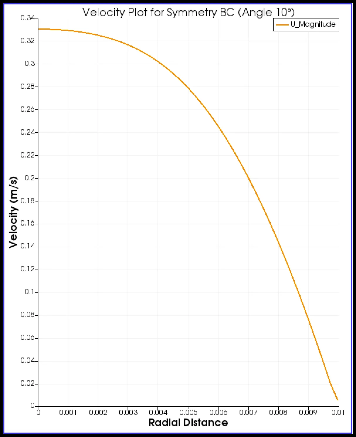
Velocity profile
Pressure profile
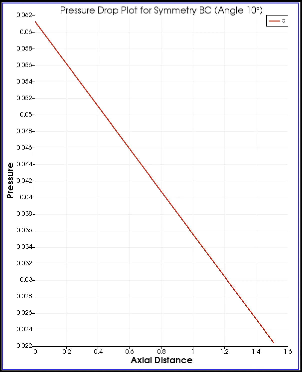
Pressure drop = (0.0612-0.0224)=0.0388
For symmetry boundary conditions
For angle 25 degrees the blockMeshDict file
 /*---------------------------------*- C++ -*-------------------------------------------------*\
 | ==========      |                                                                           |
 | \\        /  F ield        | OpenFOAM: The Open Source CFD Toolbox                          |
 |  \\      /   O peration    | Version:  9                                                    |
 |   \\    /    A nd          | Web:      www.OpenFOAM.org                                     |
 |    \\  /     M anipulation |                                                                |
  \*------------------------------------------------------------------------------------------*/
 FoamFile
{
     format         ascii;
     class          dictionary;
     object         blockMeshDict;
}
 // * * * * * * * * * * * * * * * * * * * * * * * * * * * * * * * * * * * * * * * * * * * * *  \\

convertToMeters 1;

vertices
(
      (0.000000 0.000000 0.000000)
      (0.002164 0.009763 0.000000)
      (-0.002164 0.009763 0.000000)
      (0.000000 0.000000 3.020000)
      (0.002164 0.009763 3.020000)
      (-0.002164 0.009763 3.020000)
);

blocks
(
      hex (0 0 1 2 3 3 4 5) (1 40 500) simpleGrading (1 1 1)
);

edges
(
      arc 1 2 (0.000000 0.010000 0.000000)
      arc 4 5 (0.000000 0.010000 3.020000)
);

boundary
(
      inflow
      {
           type patch;
           faces
           (
                (0 0 2 1)
           );
      }
      outflow
      {
           type patch;
           faces
           (
                (3 4 5 3)
           );
      }
      front
      {
           type symmetry;
           faces
           (
                (0 1 4 3)
           );
      }
      back
      {
           type symmetry;
           faces
           (
                (3 5 2 0)
           );
      }
      wall
      {
           type wall;
           faces
           (
                 (4 1 2 5)
           );
      }
      axis
      {
           type empty;
           faces
           (
                 (0 3 3 0)
           );
      }
);

mergePatchPairs
(
);

// ************************************************************************************************************************************************** //
Results:
blockMesh
Velocity profile
Pressure profile
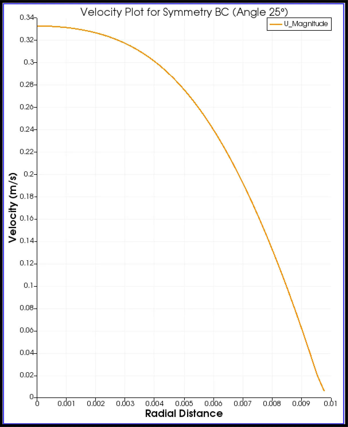
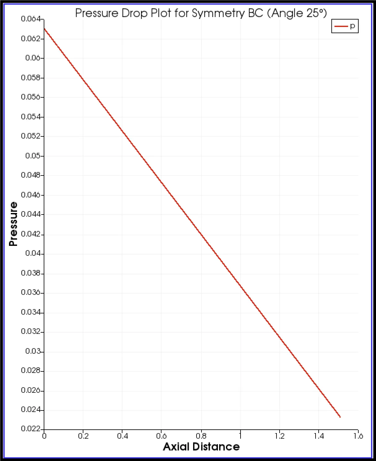
Pressure drop = (0.063-0.023)=0.043
For symmetry boundary conditions
For angle 45 degrees the blockMeshDict file
 /*---------------------------------*- C++ -*-------------------------------------------------*\
 | ==========      |                                                                           |
 | \\        /  F ield        | OpenFOAM: The Open Source CFD Toolbox                          |
 |  \\      /   O peration    | Version:  9                                                    |
 |   \\    /    A nd          | Web:      www.OpenFOAM.org                                     |
 |    \\  /     M anipulation |                                                                |
  \*------------------------------------------------------------------------------------------*/
 FoamFile
{
     format         ascii;
     class          dictionary;
     object         blockMeshDict;
}
 // * * * * * * * * * * * * * * * * * * * * * * * * * * * * * * * * * * * * * * * * * * * * *  \\

convertToMeters 1;

vertices
(
      (0.000000 0.000000 0.000000)
      (0.003827 0.009239 0.000000)
      (-0.003827 0.009239 0.000000)
      (0.000000 0.000000 3.020000)
      (0.003827 0.009239 3.020000)
      (-0.003827 0.009239 3.020000)
);

blocks
(
      hex (0 0 1 2 3 3 4 5) (1 40 500) simpleGrading (1 1 1)
);

edges
(
      arc 1 2 (0.000000 0.010000 0.000000)
      arc 4 5 (0.000000 0.010000 3.020000)
);

boundary
(
      inflow
      {
           type patch;
           faces
           (
                (0 0 2 1)
           );
      }
      outflow
      {
           type patch;
           faces
           (
                (3 4 5 3)
           );
      }
      front
      {
           type symmetry;
           faces
           (
                (0 1 4 3)
           );
      }
      back
      {
           type symmetry;
           faces
           (
                (3 5 2 0)
           );
      }
      wall
      {
           type wall;
           faces
           (
                 (4 1 2 5)
           );
      }
      axis
      {
           type empty;
           faces
           (
                 (0 3 3 0)
           );
      }
);

mergePatchPairs
(
);

// ************************************************************************************************************************************************** //
Results:
blockMesh
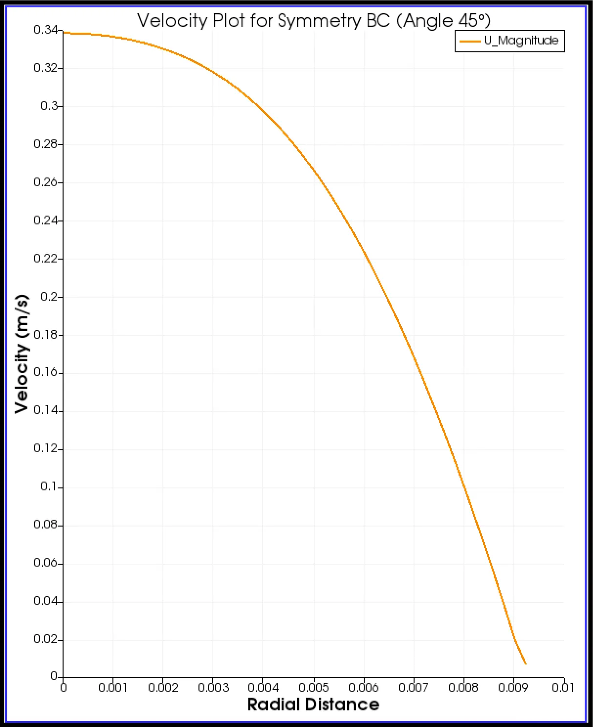
Velocity profile
Pressure profile
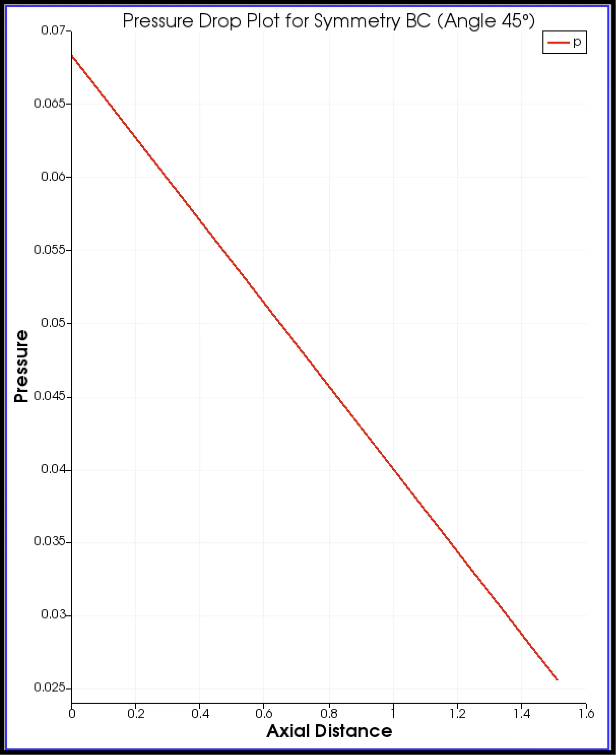
Pressure drop = (0.0683-0.0256)=0.0427
Result:
1. The first simulation comparison is with the Wedge Boundary condition. Within this Boundary Condition, the simulation comparison for all the above-mentioned angles is as follows.
We will compare the Shear Stress developed for both the boundary conditions at all three angles.
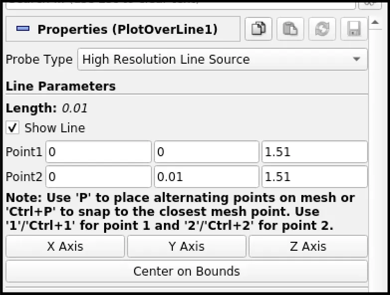
a.Shear Stress Variation with respect to the Radial Distance.
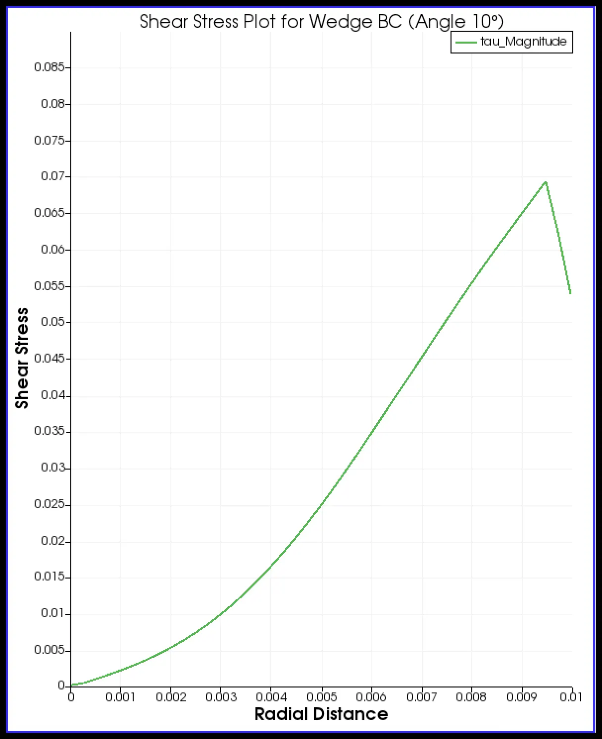
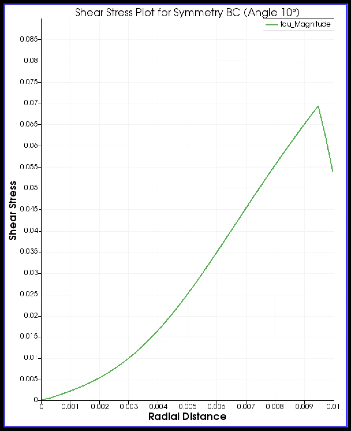
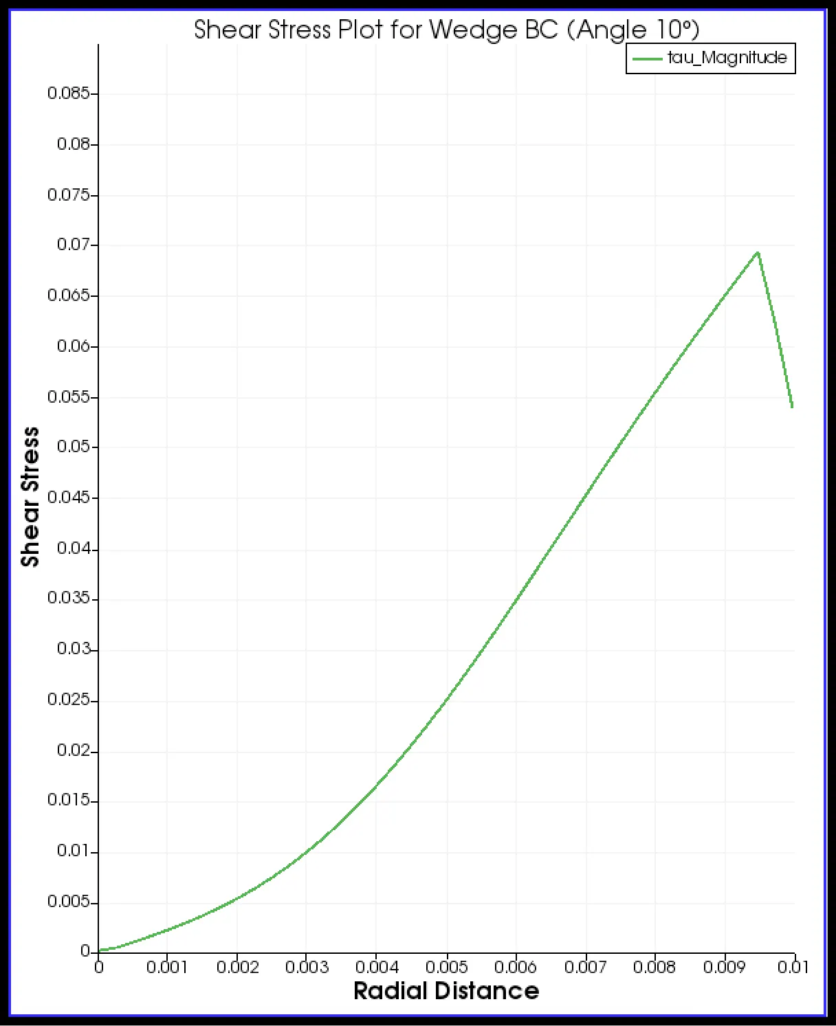
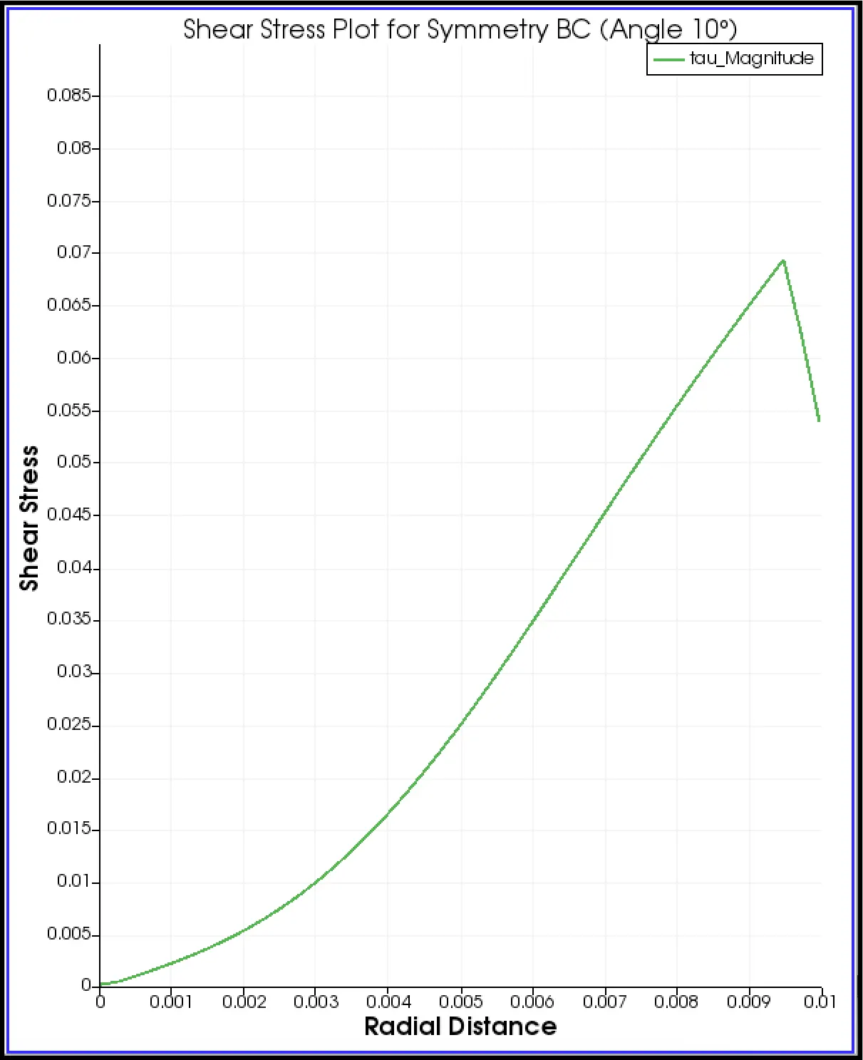
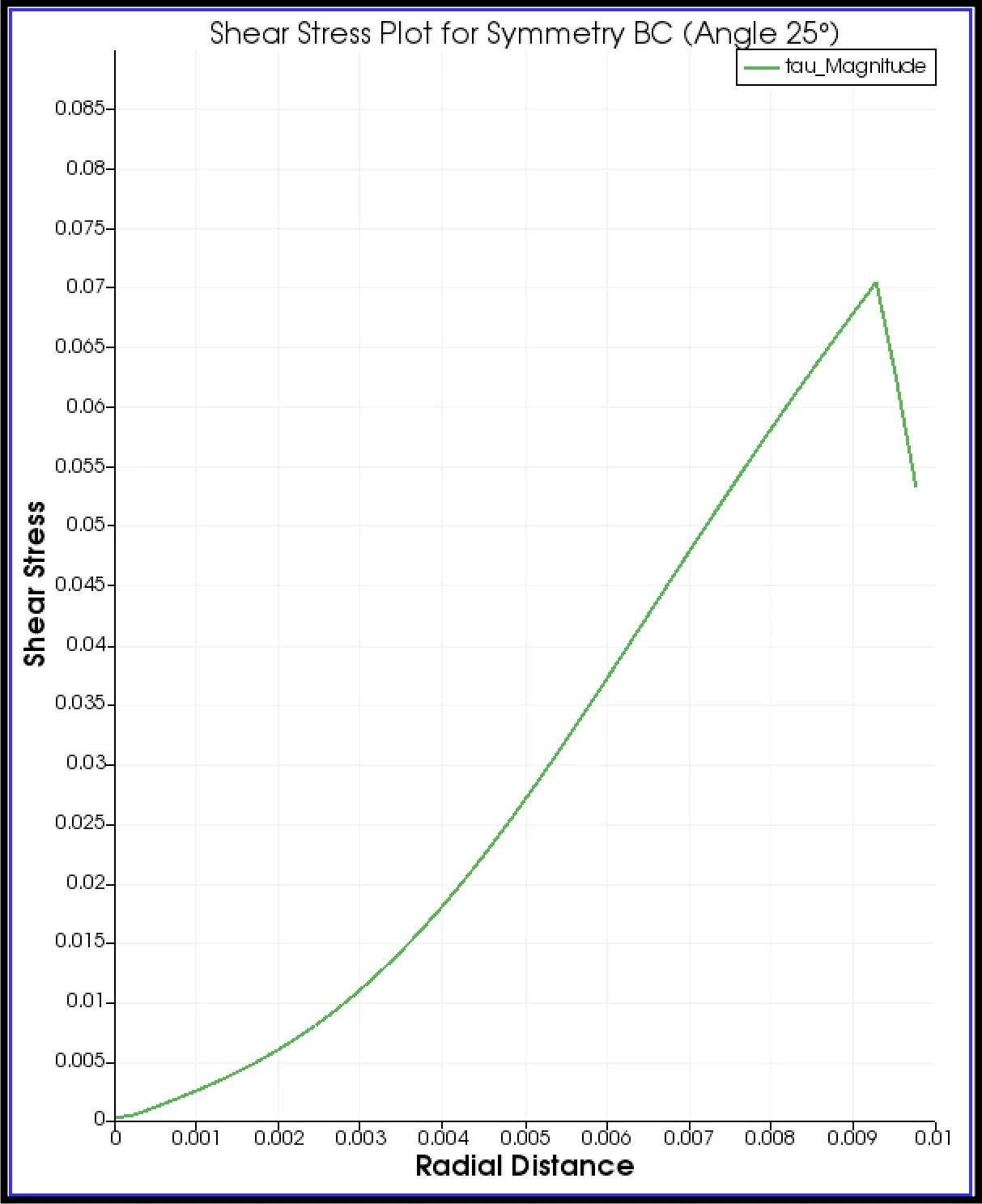
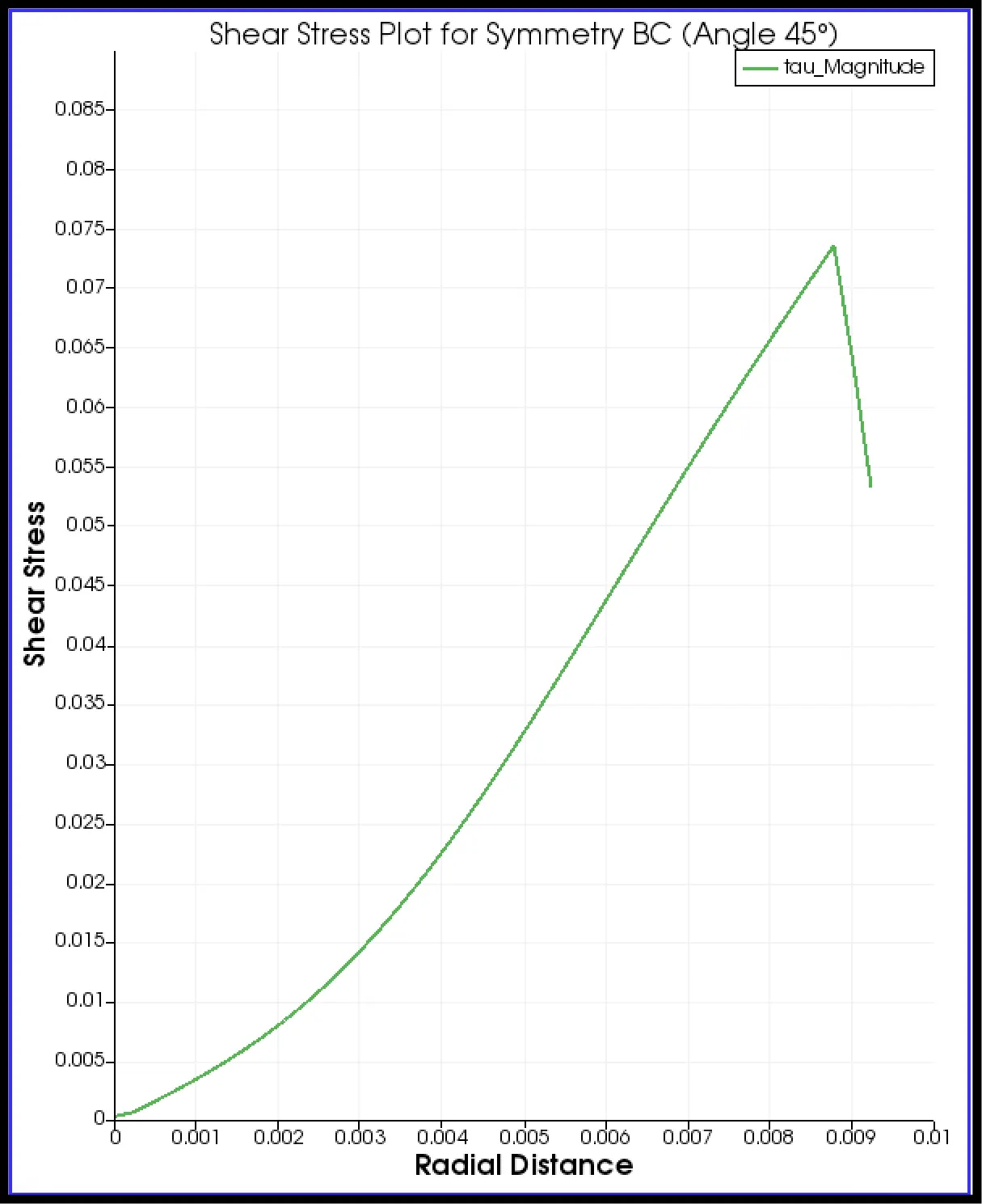
The Shear Stress plot for both the Boundary Conditions, the wedge Boundary Condition and the Symmetry Boundary Condition are shown at 10degrees. We can see that when we apply the Symmetry Boundary Condition, the slope of the curve is much higher than when we apply the Wedge Boundary Condition. So, when we apply the Symmetry Boundary Condition, the Mesh becomes 3D, and the computation is done for all three global axes. This affects the calculation as well. The peak value in the Wedge Boundary Condition is approximately 0.068units, but whereas when we apply the Symmetry Boundary Condition, the peak value touches around 0.068units.
The graph shown above is comparing the Shear Stress for both the boundary conditions for when the wedge angle is 25degrees.
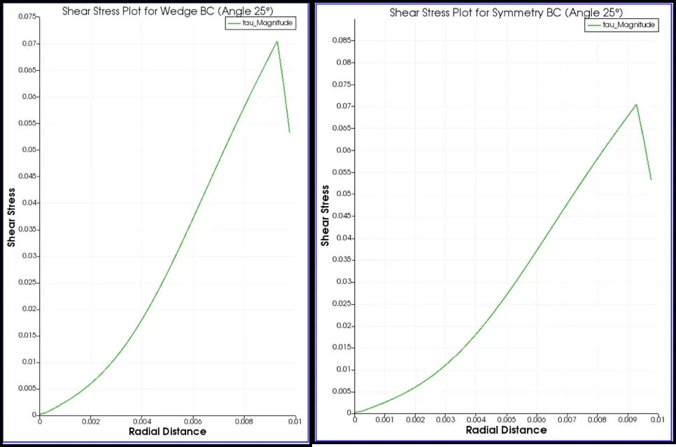
Similarly, we plot and study all the graphs, as shown below:
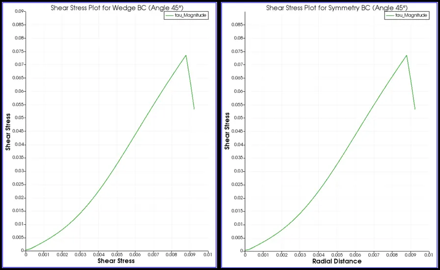
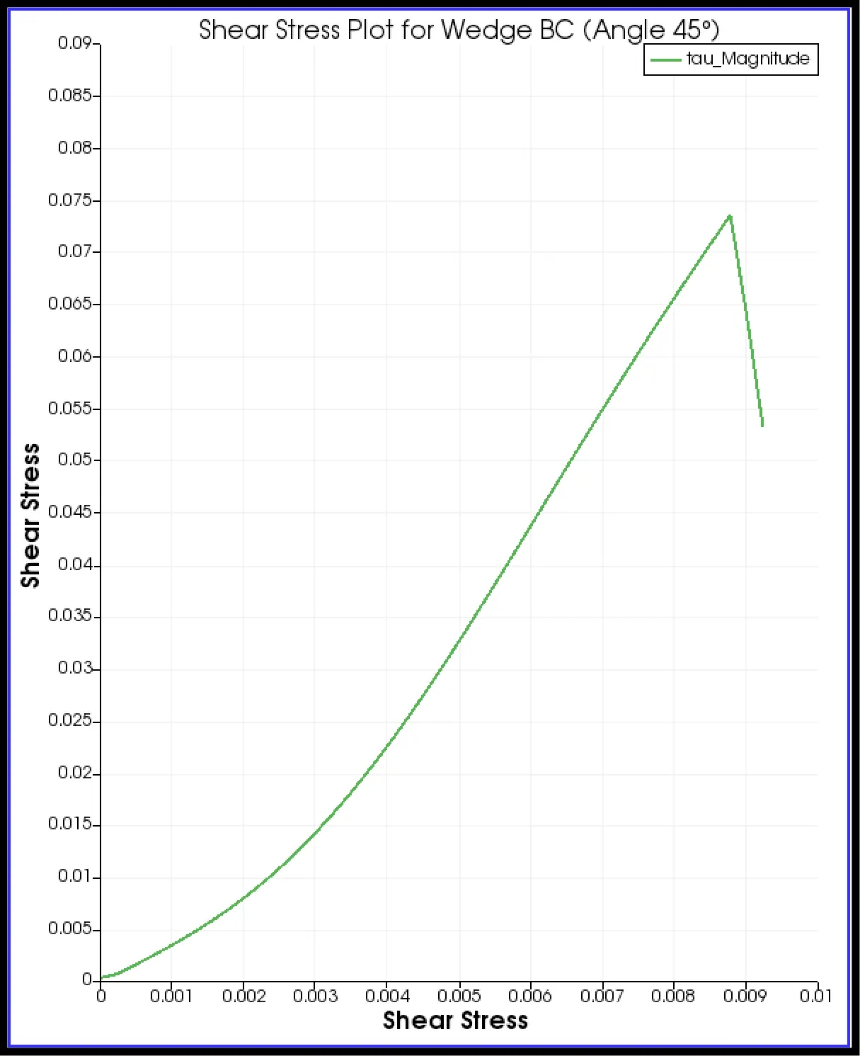
This graph compares the Shear Stress at 45 Deg for both the Boundary conditions.
b. Velocity Variation with respect to Radial Distance.
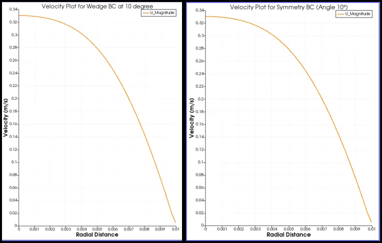
Velocity variation at 10° for the two Boundary Conditions.
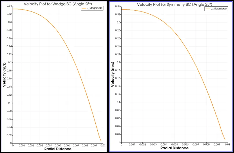
Velocity variation at 25° for the two Boundary Conditions.
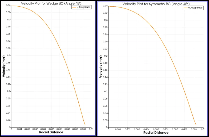
Velocity variation at 45° for the two Boundary Conditions.
c. Pressure Drop across the axial Distance
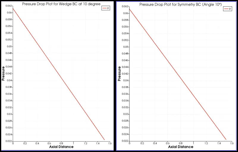
Pressure drop at 10 ° across the Axial Distance. Pressure drop = (0.061-0.023)=0.038
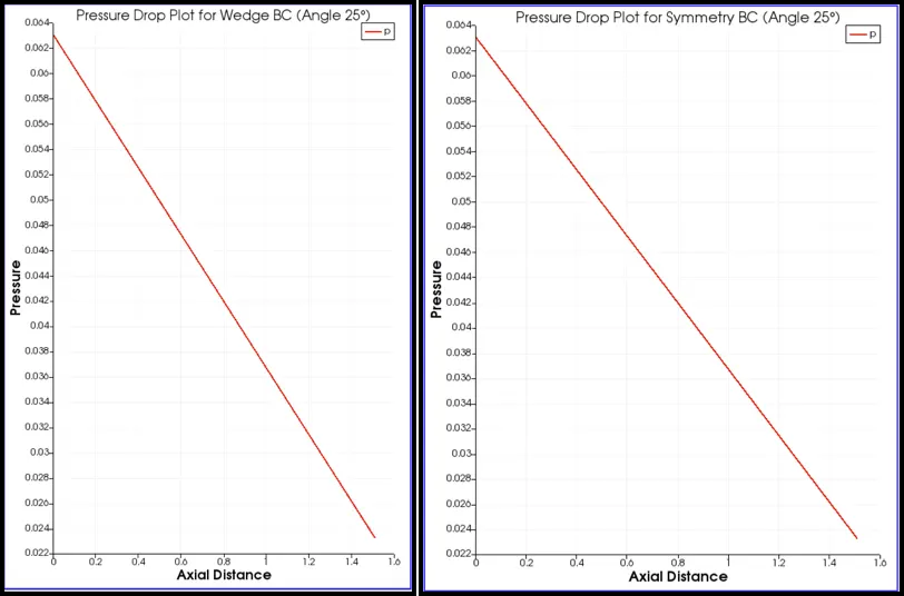
Pressure drop at 25 ° across the Axial Distance. Pressure drop = (0.063-0.023)=0.043
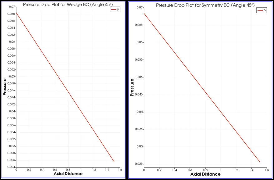
Pressure drop at 45° across the Axial Distance. Pressure drop = (0.0683-0.0256)=0.0427
Validation:
a.Validation of Maximum Pressure drop in the Fully developed Region.
These graphs depict the change in the various parameters for both the Boundary Conditions, and we can compare these quantities properly.
Like for example, we can compare the pressure drop from the graph and the pressure drop that we get analytically.
From the graph, we can see that the
maximum value - minimum value = Pressure drop = (0.061-0.023)=0.038units = 3.8 Pascal.
And, when we calculate it analytically, we know that the formula is :
ΔP =Ploss=32μ(L−Le)Vavg/D2ℎ
Here
Vavg = Average velocity
Vmax = maximum velocity
τmax = maximum shear stress
μ = dynamic viscosity
Dℎ = hydraulic diameter of the pipe
rℎ= hydraulic radius of the pipe
Ploss = pressure loss
Le = Entrance Length = 0.06 Re Dℎ (For laminar flow through a circular pipe)
kinematic pressure drop=ΔP /ρ
We know all the values, they are as follows:
% inputs
% assumptions made the fluid is assumed as water
Re=2100; % given Reynolds number
rho=997; �nsity of the water kg/m^3
D=0.02; % diameter of the pipe m
r=D/2; % radius of the pipe
mu=0.89*10^-3; % dynamic viscosity of the water at 25 degree celsius
v=0.8927*10^-6; % kinematic viscosity of the water at 25 degree celsius
Le=0.06*Re*D; % hydrodynamic length
L=Le+0.5;
theta=input('Enter the value of the wedge angle = ')
% Analytical solutions
V_avg=(Re*mu)/(rho*D); % average velocity
V_max=2*V_avg; % maximum velocity
P_drop=(32*mu*L*V_avg)/D^2; % pressure drop
P_kinematic=(P_drop)/rho; % kinematic pressure drop
For a Kinematic Viscosity of 0.88927*10^-6(Used in the simulation), the
μ=Dynamic Viscosity is 0.88927*10^-6*1000 = 0.00089 units.
Calculating using these values, we get: ΔP =Ploss=32μ(L-Le)V_avg/D2ℎ
V_avg=(Re*mu)/(rho*D);
= (2100 * 0.00089)/(997 * 0.02)
= 0.09373 m/s
Le=0.06*Re*D; % hydrodynamic length
= 0.06 * 2100* 0.02 = 2.52 m
L = Le + 0.5= 2.52+0.5=3.02
ΔP = (32 * 0.00089*0.5*0.09373)/(0.02)^2 = 0.0013347152/0.0004
=3.336788
P_kinematic=(P_drop)/rho; % kinematic pressure drop
= 3.336/997
=0.003346038114343
The error between the Analytical value and the value obtained from the graph is (3.8-3.336) / (3.336) = 0.14%, which is under the tolerance limit of 5%.
Now, because the error is under tolerance, we can conclude that the simulation has reached a Steady State.
b.Validation of the Maximum Velocity
Now, if we wish to compare the Maximum velocity from the graph, we can see that the value is 0.31 units.
According to the Analytical formula, we know that the maximum velocity must be: V_avg *2
And our V_avg = 0.1875 units
hence the analytical value will be 0.3748 units that matches the value that we get from the graph.
c. To validate the Hydrodynamic length with the Numerical Result.
So, In fluid dynamics, the entrance length is the distance a flow travels after entering a pipe before the flow becomes fully developed. Entrance length refers to the length of the entry region, the area following the pipe entrance where effects originating from the interior wall of the pipe propagate into the flow as an expanding boundary layer.
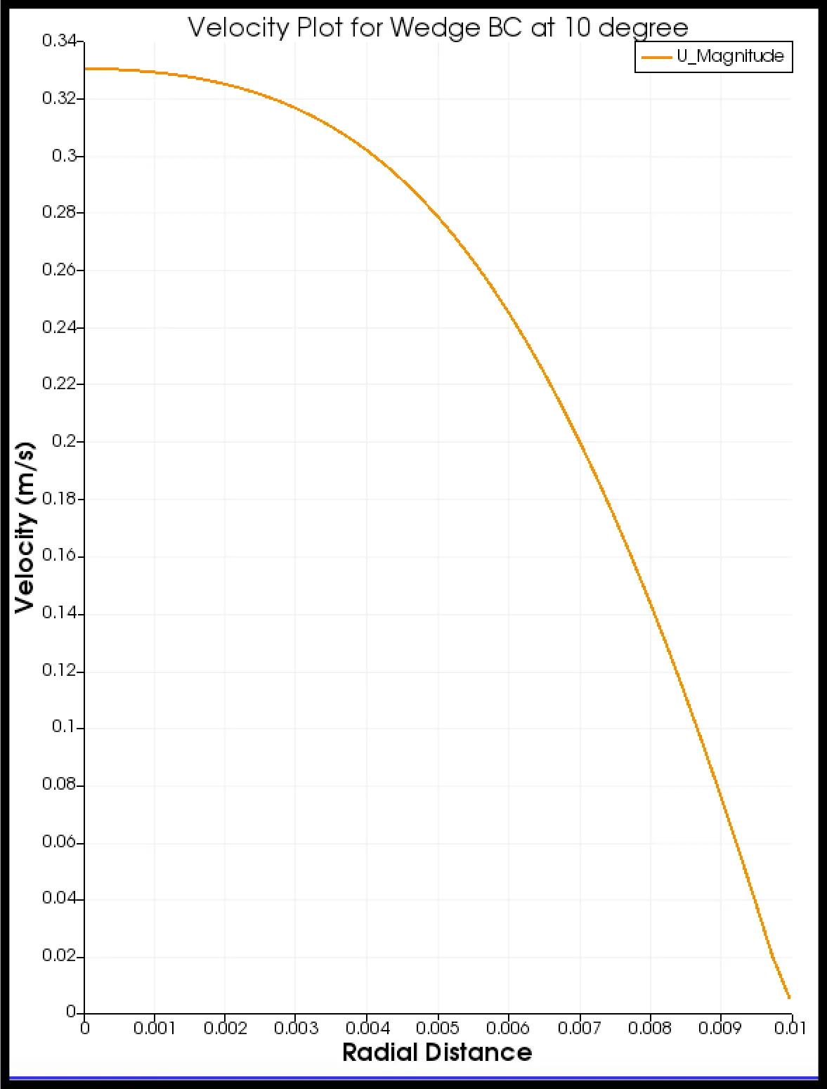
Here, numerically, we know that the velocity profile will be different before and after the Hydrodynamic entry length. After the Hydrodynamic entry length, the Velocity profile will be the final parabolic profile that it must have in a fully developed region.
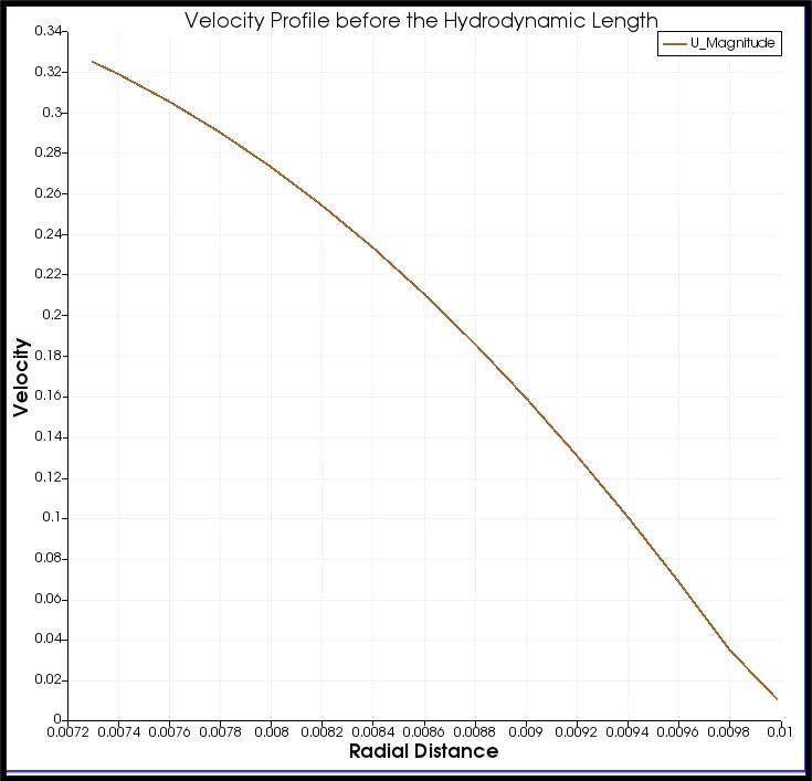
Velocity profile before the Hydrodynamic Length
Here is the velocity profile before the Hydrodynamic Length. We can see that this plot is not properly parabolic.
The location where the velocity was measured for the above plot:
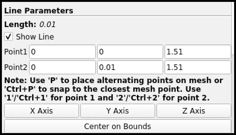
Whereas, if we compare the velocity profile at a location after the hydrodynamic length and in the fully developed region, the velocity profile will be much more defined and proper.
Velocity after the Hydrodynamic length
The location where the velocity was measured for the above plot:
Now, If we wish to calculate the Hydrodynamic length analytically, the formula is as follows:
Le = 0.6*Re *D
where:
Re = Reynolds number.
D = Diameter.
In our case, Re = 2100 and the Diameter = 0.02m, so the Hydrodynamic Length is:
Le = 0.06*2100*0.02 = 2.52m.
And from the two graphs above, we can confirm that only after the Hydrodynamic length of approximately 2.5m, the velocity profile is changing into a fully parabolic shape.
d. Shear Stress Plot:
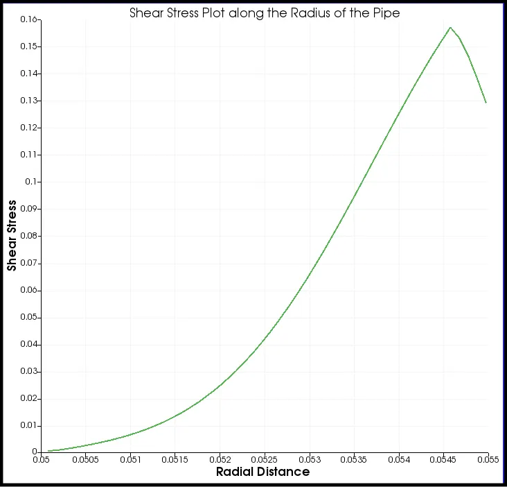
Shear Stress Plot
Shear Stress is the maximum near the wall because of the friction that the wall has. But, as we move away from the wall, the Shear Force decreases, and it can be confirmed with the graph above.
According to the Analytically calculated profile, the graph is:
u(r) = 2 * V_avg *(1-(r^2/R^2))
And we know that this profile also gives out a Parabolic curve similar to the one we have gotten in the graph.
e. Comparison between the two Boundary Conditions.
We have performed Simulation for two Boundary Conditions; those are Symmetry Boundary Condition and the Wedge Boundary Condition.
During the Wedge Boundary condition simulation, the simulation across the arc of the wedge is not done, but whereas in the case of Symmetry Boundary Condition, the calculation across the arc of the wedge is done; hence the simulation time is higher in that case. The Courant number is increasing slightly in the case of wedge Boundary Condition and hence the Symmetry Boundary Condition will be slightly more accurate. The Symmetry Boundary condition considers the Mesh as 3D and the calculation is done along all the three global axes.
We understand the results should not change due to the change in the Boundary conditions, and this is because the Physics of the problem does not change and remains the same.
Conclusion: In conclusion, I would like to state that this challenge helped me understand the difference between the two boundary conditions and how to simulate them as per the need of the problem that we will be simulating.