Week 12 - Validation studies of Symmetry BC vs Wedge BC in OpenFOAM vs Analytical H.P equation
Title : Validation studies of Symmetry BC vs Wedge BC in OpenFOAM vs Analytical H.P equation
Objectives :
- Simulate the laminar flow through constant cross-section of the pipe problem by applying both Wedge and Symmetry boundary Condition
- Simulate the problem for three different wedge angle `10^(circ) ,25^(circ) and 45^(circ)`
- Validate the fully developed flow velocity profile with its analytical profile
- Validate maximum velocity and pressured drop for fully developed flow
- Post-process Shear stress and validate wall shear stress for fully developed flow
- Comment on the difference between the two different boundary conditions
ABSTRACT
Hagen–Poiseuille equation, also known as the Hagen–Poiseuille law, Poiseuille law or Poiseuille equation, is a physical law that gives the pressure drop in an incompressible and Newtonian fluid in laminar flow flowing through a long cylindrical pipe of constant cross section. It can be successfully applied to air flow in lung alveoli, or the flow through a drinking straw. It was experimentally derived independently by Jean Léonard Marie Poiseuille in 1838 and Gotthilf Heinrich Ludwig Hagen, and published by Poiseuille in 1840–41 and 1846. The theoretical justification of the Poiseuille law was given by George Stokes in 1845. This project presents the simulation of Hagen–Poiseuille Flow (Laminar-Incompressible Flow) through a pipe having constant circular cross-section throughout the length.
The whole report can be divided into two sections; The former part aims to implement automation in the generation of computational mesh file, time-control file, and other necessary script files (later, these will be used by OpenFOAM to run the simulation) using MATLAB. As the flow has axis-symmetrical nature, only a reduced model (Wedge) is considered instead of entire circular pipe, thus reducing computational efforts extensively. A suitable wedge angle is considered to simulate the flow realistically. In the final section, the CFD analysis is carried out with an open-source CFD toolbox called OpenFOAM, which makes use of all of the script files that have already been generated. The primary focus of this project is to investigate the evolution of the velocity profile in the Hydrodynamic Entrance Region and the variation in shear stress along the pipe's axial direction. Also to study the difference between symmetry boundary condition and wedge boundary condition. In order to guarantee the accuracy of the numerical results, the obtained CFD data are validated using analytical values derived from the Hagen–Poiseuille equations during this project.
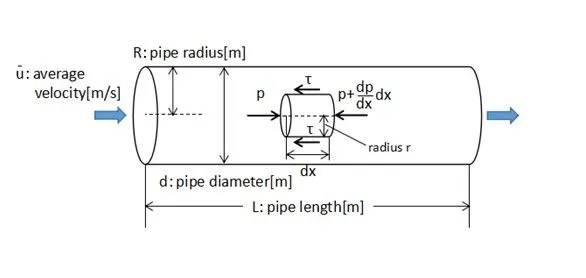
Hagen - Poiseuille flow
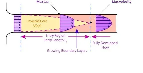
As soon as the fluid enters the circular pipe with a certain constant velocity, an axisymmetric velocity boundary layer is established at the pipe wall. A boundary layer is a thin layer of viscous fluid close to the solid surface of a wall in contact with a moving stream in which the flow velocity varies from zero at the wall (where the flow “sticks” to the wall because of its viscosity) up to free stream velocity at the boundary. Initially, the flow is in the undeveloped state; as the fluid travels further axially into the pipe, the velocity profile keeps continuously changing, and the boundary layer grows and eventually reaches the center of the pipe. This change in the velocity profile occurs due to the generation of net shear stress between different layers of the fluid.
Beyond the axia location flow is said to be fully developed. Fully-developed flow is what we call it when the velocity profile does not change along the direction of flow (axial direction). The developing flow becomes a fully developed flow, where flow characteristics no longer change with increased distance along the pipe. The entrance length is the distance a flow travels after entering a pipe before the flow becomes fully developed.
The hydrodynamic entrance region refers to the area of a pipe where fluid entering a pipe develops a velocity profile due to viscous forces propagating from the interior wall of a pipe. The fluid enters a pipe at a uniform velocity, then fluid particles in the layer in contact with the surface of the pipe come to a complete stop due to the no-slip condition. Due to viscous forces within the fluid, the layer in contact with the pipe surface resists the motion of adjacent layers and slows adjacent layers of fluid down gradually, forming a velocity profile. It should be noted that the Hagen–Poiseuille equation applies only to laminar flows in a pipe.
Hagen–Poiseuille equation
Poiseuille's equation describes the pressure drop due to the viscosity of the fluid. The Hagen–Poiseuille Equation (or Poiseuille equation) is a fluidic law to calculate flow pressure drop in a long cylindrical pipe.
Assumptions of the Hagen–Poiseuille equation
- Fluid is incompressible and Newtonian
- The flow is laminar through a pipe of constant circular cross-section
- No acceleration of fluid in the pipe
- For velocities and pipe diameters above a threshold, actual fluid flow is not laminar but turbulent, leading to larger pressure drops
Importance equations and analytical solutions : Now, we are going to describe some essential flow equation which will be needed to calculate the analytical solution of this physical flow model. These analytical solutions will then use to validate the obtained CFD values at the end of the report, to assure the fidelity of the numerical results.
Reynolds number = inertia force / voscous force
= `Re=(rhoDV_[avg])/(mu)`
Velocity at the location where the boundary layer is fully developed `= U ( r ) = 2 V_(a v g) ( 1 − r^2 /R ^2 )`
Pressure drop through the length of pipe p1-p2 = `DeltaP=(32muLV_[avg])/D^2`
Entrance length for laminar flow , `L_e = 0.06*Re*D`
Shear stress ( Represented by velocity gradient perpendicular to flow direction), `tau = mu*(delu)/(dely)`
where ,`mu`= dynamic viscosity of the liquid
L = length of the pipe
R = radius of the pipe
D = diameter of the pipe
`tau` = shear-stress
Geometry and Mesh generation
The figure below will give an overview of our domain and geometry that are going to be used in further analysis.
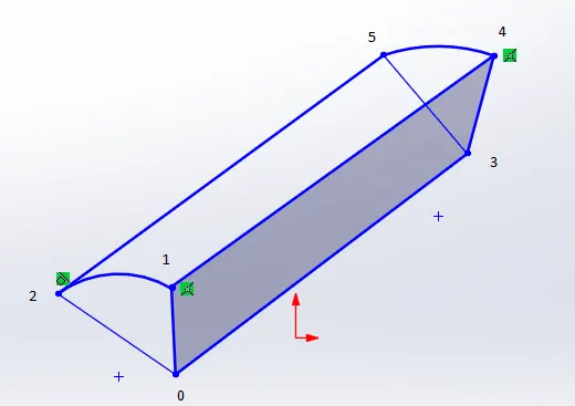
1. The procedure for this challenge involves editing the previously made MATLAB code and changing the input and the Boundary Conditions in OpenFoam.
2. In the Automated BlockMeshDict file, we need to edit the wedge angle for one particular boundary condition. The angles at which we are performing the simulation and then later studying the simulation results are:
- `10^(circ)`
- `25^(circ)`
- `45^(circ)`
Wedge boundary condition : The wedge boundary condition is used in computational fluid dynamics to define an axisymmetric situation, for eg. a cylinder. The model and flow must be axisymmetric along a central line such that all physical variables of the flow have the same value and distribution at a given radius for all angles.
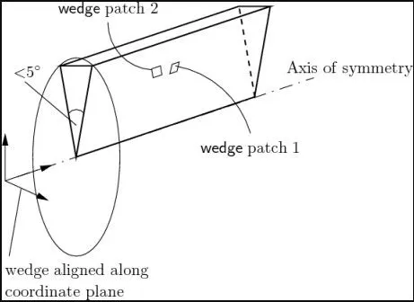
Symmetry boundary condition : The symmetry boundary condition defines a mirror face/surface.
MATLAB code for wedge boundary condition at a wedge angle of `10^(circ)`
clear all        %Clear all existing  variables from workspace
close all        %Close the figure windows
clc              %Clear the command window

%% inputs
Re=2100;
%length of the pipe
L=3;
%Diameter of the pipe
D=0.02;
theta= 10;       %Wedge angle
rho=997;         %Density of the working fluid (water)
mu=0.892*1e-3;   %Dynamic viscosity of water
R=D/2;

L_e= 0.058*Re*D; %Caculating the entrance length

%Simple grading along X,Y and Z directions
meshx=20;
meshy=500;
meshz=1;
gradex=1;
gradey=0.2;
gradez=1;

V_avg= (Re*mu)/(rho*D);
V_max= 2*V_avg;
delta_p=(32*mu*L*V_avg)/(D^2);
kin_p=(delta_p)/(rho);

%% determining the vertices of wedge
v0=[0,0,0];
v1=[0,(R*cosd(theta/2)),(R*sind(theta/2))];
v2=[0,(R*cosd(theta/2)),(-R*sind(theta/2))];
v3=[L,0,0];
v4=[L,(R*cosd(theta/2)),(R*sind(theta/2))];
v5=[L,(R*cosd(theta/2)),-(R*sind(theta/2))];

%% Writing the blockmechdict file
f1=fopen('blockMeshDict.txt','w');

fprintf(f1,'%s','/--------------------------------- C++ -----------------------------------');
fprintf(f1,'\n=========              | ');
fprintf(f1,'\n\\      /  F ield      | OpenFOAM: The Open Source CFD Toolbox');
fprintf(f1,'\n \\    /   O peration   | Website:  https://openfoam.org');
fprintf(f1,'\n  \\  /    A nd          | Version:  10');
fprintf(f1,'\n   \\/     M anipulation  |');
fprintf(f1,'\n*---------------------------------------------------------------------------*/');
fprintf(f1,'\nFoamFile');
fprintf(f1,'\n{');
fprintf(f1,'\nformat      ascii;')
fprintf(f1,'\nclass       dictionary;')
fprintf(f1,'\nobject      blockMeshDict;')
fprintf(f1,'\n}');
fprintf(f1,'\n%s','// * * * * * * * * * * * * * * * * * * * * * * * * * * * * * * * * * * * * * //');
fprintf(f1,'\nconvertToMeters 1;');
fprintf(f1,'\nvertices');
fprintf(f1,'\n(');
fprintf(f1,'\n(%f %f %f)//point0',v0(1),v0(2),v0(3));
fprintf(f1,'\n(%f %f %f)//point1',v1(1),v1(2),v1(3));
fprintf(f1,'\n(%f %f %f)//point2',v2(1),v2(2),v2(3));
fprintf(f1,'\n(%f %f %f)//point3',v3(1),v3(2),v3(3));
fprintf(f1,'\n(%f %f %f)//point4',v4(1),v4(2),v4(3));
fprintf(f1,'\n(%f %f %f)//point5',v5(1),v5(2),v5(3));
fprintf(f1,'\n);');
fprintf(f1,'\nblocks');
fprintf(f1,'\n(');
fprintf(f1,'\n hex (0 1 4 3 0 2 5 3) (%d %d %d ) simpleGrading (%f %f %f)',meshx,meshy,meshz,gradey,gradex,gradez);
fprintf(f1,');');
fprintf(f1,'\nedges');
fprintf(f1,'\n(');
fprintf(f1,'\n arc 2 1 (%f %f %f)',0,R,0);
fprintf(f1,'\n arc 5 4 (%f %f %f)',L,R,0);
fprintf(f1,'\n);');

fprintf(f1,'\nboundary');
fprintf(f1,'\n(');
fprintf(f1,'\n    inlet');
fprintf(f1,'\n    {');
fprintf(f1,'\n	type patch;');
fprintf(f1,'\n	faces');
fprintf(f1,'\n	(');
fprintf(f1,'\n 	(0 1 2 0)');
fprintf(f1,'\n 	);');
fprintf(f1,'\n    }');
fprintf(f1,'\n    outlet');
fprintf(f1,'\n    {');
fprintf(f1,'\n	type patch;');
fprintf(f1,'\n	faces');
fprintf(f1,'\n	(');
fprintf(f1,'\n	(3 5 4 3)');
fprintf(f1,'\n	);');
fprintf(f1,'\n    }');
fprintf(f1,'\n    topwall');
fprintf(f1,'\n    {');
fprintf(f1,'\n	type wall;');
fprintf(f1,'\n	faces');
fprintf(f1,'\n 	(');
fprintf(f1,'\n	(1 4 5 2)');
fprintf(f1,'\n	);');
fprintf(f1,'\n    }');
fprintf(f1,'\n    front');
fprintf(f1,'\n    {');
fprintf(f1,'\n	type wedge;');
fprintf(f1,'\n	faces');
fprintf(f1,'\n	(');
fprintf(f1,'\n	(0 3 4 1)');
fprintf(f1,'\n	);');
fprintf(f1,'\n    }');
fprintf(f1,'\n    back');
fprintf(f1,'\n    {');
fprintf(f1,'\n 	type wedge;');
fprintf(f1,'\n	faces');
fprintf(f1,'\n 	(');
fprintf(f1,'\n 	(0 2 5 3)');
fprintf(f1,'\n	);');
fprintf(f1,'\n    }');
fprintf(f1,'\n    axis');
fprintf(f1,'\n    {');
fprintf(f1,'\n	type empty;');
fprintf(f1,'\n	faces');
fprintf(f1,'\n	(');
fprintf(f1,'\n	(0 3 3 0)');
fprintf(f1,'\n	);');
fprintf(f1,'\n    }');
fprintf(f1,'\n);');


fprintf(f1,'\nmergePatchPairs');
fprintf(f1,'\n(');
fprintf(f1,'\n);');
fprintf(f1,'\n// ************************************************************************* //');
MATLAB code for symmetry boundary condition at a wedge angle of `10^(circ)`
clear all        %Clear all existing  variables from workspace
close all        %Close the figure windows
clc              %Clear the command window

%% inputs
Re=2100;
%length of the pipe
L=3;
%Diameter of the pipe
D=0.02;
theta= 10;       %Wedge angle
rho=997;         %Density of the working fluid (water)
mu=0.892*1e-3;   %Dynamic viscosity of water
R=D/2;

L_e= 0.058*Re*D; %Caculating the entrance length

%Simple grading along X,Y and Z directions
meshx=20;
meshy=500;
meshz=1;
gradex=1;
gradey=0.2;
gradez=1;

V_avg= (Re*mu)/(rho*D);
V_max= 2*V_avg;
delta_p=(32*mu*L*V_avg)/(D^2);
kin_p=(delta_p)/(rho);

%% determining the vertices of wedge
v0=[0,0,0];
v1=[0,(R*cosd(theta/2)),(R*sind(theta/2))];
v2=[0,(R*cosd(theta/2)),(-R*sind(theta/2))];
v3=[L,0,0];
v4=[L,(R*cosd(theta/2)),(R*sind(theta/2))];
v5=[L,(R*cosd(theta/2)),-(R*sind(theta/2))];

%% Writing the blockmechdict file
f1=fopen('blockMeshDict.txt','w');

fprintf(f1,'%s','/--------------------------------- C++ -----------------------------------');
fprintf(f1,'\n=========              | ');
fprintf(f1,'\n\\      /  F ield      | OpenFOAM: The Open Source CFD Toolbox');
fprintf(f1,'\n \\    /   O peration   | Website:  https://openfoam.org');
fprintf(f1,'\n  \\  /    A nd          | Version:  10');
fprintf(f1,'\n   \\/     M anipulation  |');
fprintf(f1,'\n*---------------------------------------------------------------------------*/');
fprintf(f1,'\nFoamFile');
fprintf(f1,'\n{');
fprintf(f1,'\nformat      ascii;')
fprintf(f1,'\nclass       dictionary;')
fprintf(f1,'\nobject      blockMeshDict;')
fprintf(f1,'\n}');
fprintf(f1,'\n%s','// * * * * * * * * * * * * * * * * * * * * * * * * * * * * * * * * * * * * * //');
fprintf(f1,'\nconvertToMeters 1;');
fprintf(f1,'\nvertices');
fprintf(f1,'\n(');
fprintf(f1,'\n(%f %f %f)//point0',v0(1),v0(2),v0(3));
fprintf(f1,'\n(%f %f %f)//point1',v1(1),v1(2),v1(3));
fprintf(f1,'\n(%f %f %f)//point2',v2(1),v2(2),v2(3));
fprintf(f1,'\n(%f %f %f)//point3',v3(1),v3(2),v3(3));
fprintf(f1,'\n(%f %f %f)//point4',v4(1),v4(2),v4(3));
fprintf(f1,'\n(%f %f %f)//point5',v5(1),v5(2),v5(3));
fprintf(f1,'\n);');
fprintf(f1,'\nblocks');
fprintf(f1,'\n(');
fprintf(f1,'\n hex (0 1 4 3 0 2 5 3) (%d %d %d ) simpleGrading (%f %f %f)',meshx,meshy,meshz,gradey,gradex,gradez);
fprintf(f1,');');
fprintf(f1,'\nedges');
fprintf(f1,'\n(');
fprintf(f1,'\n arc 2 1 (%f %f %f)',0,R,0);
fprintf(f1,'\n arc 5 4 (%f %f %f)',L,R,0);
fprintf(f1,'\n);');

fprintf(f1,'\nboundary');
fprintf(f1,'\n(');
fprintf(f1,'\n    inlet');
fprintf(f1,'\n    {');
fprintf(f1,'\n	type patch;');
fprintf(f1,'\n	faces');
fprintf(f1,'\n	(');
fprintf(f1,'\n 	(0 1 2 0)');
fprintf(f1,'\n 	);');
fprintf(f1,'\n    }');
fprintf(f1,'\n    outlet');
fprintf(f1,'\n    {');
fprintf(f1,'\n	type patch;');
fprintf(f1,'\n	faces');
fprintf(f1,'\n	(');
fprintf(f1,'\n	(3 5 4 3)');
fprintf(f1,'\n	);');
fprintf(f1,'\n    }');
fprintf(f1,'\n    topwall');
fprintf(f1,'\n    {');
fprintf(f1,'\n	type wall;');
fprintf(f1,'\n	faces');
fprintf(f1,'\n 	(');
fprintf(f1,'\n	(1 4 5 2)');
fprintf(f1,'\n	);');
fprintf(f1,'\n    }');
fprintf(f1,'\n    front');
fprintf(f1,'\n    {');
fprintf(f1,'\n	type symmetry;');
fprintf(f1,'\n	faces');
fprintf(f1,'\n	(');
fprintf(f1,'\n	(0 3 4 1)');
fprintf(f1,'\n	);');
fprintf(f1,'\n    }');
fprintf(f1,'\n    back');
fprintf(f1,'\n    {');
fprintf(f1,'\n 	type symmetry;');
fprintf(f1,'\n	faces');
fprintf(f1,'\n 	(');
fprintf(f1,'\n 	(0 2 5 3)');
fprintf(f1,'\n	);');
fprintf(f1,'\n    }');
fprintf(f1,'\n    axis');
fprintf(f1,'\n    {');
fprintf(f1,'\n	type empty;');
fprintf(f1,'\n	faces');
fprintf(f1,'\n	(');
fprintf(f1,'\n	(0 3 3 0)');
fprintf(f1,'\n	);');
fprintf(f1,'\n    }');
fprintf(f1,'\n);');


fprintf(f1,'\nmergePatchPairs');
fprintf(f1,'\n(');
fprintf(f1,'\n);');
fprintf(f1,'\n// ************************************************************************* //');
Desired blockMeshDict file using the above MATLAB script file for wedge boundary condition at a angle of `10^(circ)`
/--------------------------------- C++ -----------------------------------
=========              |
\      /  F ield      | OpenFOAM: The Open Source CFD Toolbox
 \    /   O peration   | Website:  https://openfoam.org
  \  /    A nd          | Version:  10
   \/     M anipulation  |
*---------------------------------------------------------------------------*/
FoamFile
{
format      ascii;
class       dictionary;
object      blockMeshDict;
}
// * * * * * * * * * * * * * * * * * * * * * * * * * * * * * * * * * * * * * //
convertToMeters 1;
vertices
(
(0.000000 0.000000 0.000000)//point0
(0.000000 0.009962 0.000872)//point1
(0.000000 0.009962 -0.000872)//point2
(3.000000 0.000000 0.000000)//point3
(3.000000 0.009962 0.000872)//point4
(3.000000 0.009962 -0.000872)//point5
);
blocks
(
 hex (0 1 4 3 0 2 5 3) (20 500 1 ) simpleGrading (0.200000 1.000000 1.000000));
edges
(
 arc 2 1 (0.000000 0.010000 0.000000)
 arc 5 4 (3.000000 0.010000 0.000000)
);
boundary
(
    inlet
    {
	type patch;
	faces
	(
 	(0 1 2 0)
 	);
    }
    outlet
    {
	type patch;
	faces
	(
	(3 5 4 3)
	);
    }
    topwall
    {
	type wall;
	faces
 	(
	(1 4 5 2)
	);
    }
    front
    {
	type wedge;
	faces
	(
	(0 3 4 1)
	);
    }
    back
    {
 	type wedge;
	faces
 	(
 	(0 2 5 3)
	);
    }
    axis
    {
	type empty;
	faces
	(
	(0 3 3 0)
	);
    }
);
mergePatchPairs
(
);
// ************************************************************************* //
Desired blockMeshDict file using the above MATLAB script file for symmetry boundary condition at a angle of `10^(circ)`
/--------------------------------- C++ -----------------------------------
=========              |
\      /  F ield      | OpenFOAM: The Open Source CFD Toolbox
 \    /   O peration   | Website:  https://openfoam.org
  \  /    A nd          | Version:  10
   \/     M anipulation  |
*---------------------------------------------------------------------------*/
FoamFile
{
format      ascii;
class       dictionary;
object      blockMeshDict;
}
// * * * * * * * * * * * * * * * * * * * * * * * * * * * * * * * * * * * * * //
convertToMeters 1;
vertices
(
(0.000000 0.000000 0.000000)//point0
(0.000000 0.009962 0.000872)//point1
(0.000000 0.009962 -0.000872)//point2
(3.000000 0.000000 0.000000)//point3
(3.000000 0.009962 0.000872)//point4
(3.000000 0.009962 -0.000872)//point5
);
blocks
(
 hex (0 1 4 3 0 2 5 3) (20 500 1 ) simpleGrading (0.200000 1.000000 1.000000));
edges
(
 arc 2 1 (0.000000 0.010000 0.000000)
 arc 5 4 (3.000000 0.010000 0.000000)
);
boundary
(
    inlet
    {
	type patch;
	faces
	(
 	(0 1 2 0)
 	);
    }
    outlet
    {
	type patch;
	faces
	(
	(3 5 4 3)
	);
    }
    topwall
    {
	type wall;
	faces
 	(
	(1 4 5 2)
	);
    }
    front
    {
	type symmetry;
	faces
	(
	(0 3 4 1)
	);
    }
    back
    {
 	type symmetry;
	faces
 	(
 	(0 2 5 3)
	);
    }
    axis
    {
	type empty;
	faces
	(
	(0 3 3 0)
	);
    }
);
mergePatchPairs
(
);
// ************************************************************************* //
Note : Similarly , in order to get the blockMeshDict file for angle of `25^(circ)`and `45^(circ)` only we have to replace theta as 25 and 45 in the MATLAB script file line number 11.
The mesh is generated from a dictionary file named blockMeshDict . Located inside the constant directory. BlockMesh reads this dictionary and generates the mesh.
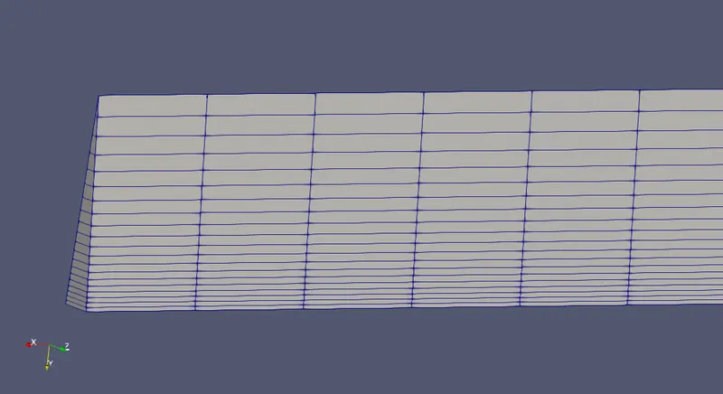
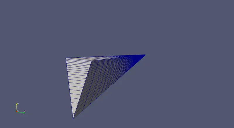
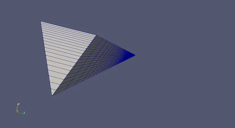
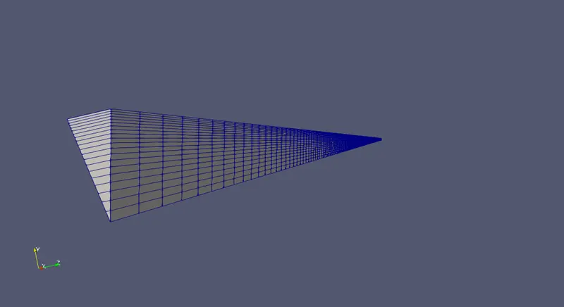
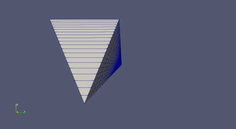
Mesh grid for Wedge boundary condition for different wedge angle `10^(circ) , 25^(circ) ,and 45^(circ)`
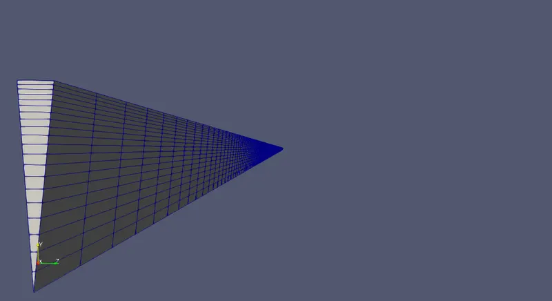
Mesh grid for symmetry boundary condition for different wedge angle `10^(circ) , 25^(circ) ,and 45^(circ)`
Specifying physical properties
In OpenFOAM, the physical parameters for a specific flow problem are described in the file called physicalProperties file. This file is located in the constant directory under our case file. In our case, we have assumed Water as a working fluid and it is a Newtonian fluid, and the kinematic viscosity of fluid flow is given as (0.0000008927 m^2/second).
PhysicalProperties file is below :
/*--------------------------------*- C++ -*----------------------------------*\
  =========                 |
  \\      /  F ield         | OpenFOAM: The Open Source CFD Toolbox
   \\    /   O peration     | Website:  https://openfoam.org
    \\  /    A nd           | Version:  10
     \\/     M anipulation  |
\*---------------------------------------------------------------------------*/
FoamFile
{
    format      ascii;
    class       dictionary;
    location    "constant";
    object      physicalProperties;
}
// * * * * * * * * * * * * * * * * * * * * * * * * * * * * * * * * * * * * * //

nu              [0 2 -1 0 0 0 0] 0.0000008927;


// ************************************************************************* //
Now, we are going to edit ‘controlDict’ file to provides time limits - start time and end time timestep size. After edting save it and close it.

controlDict file

/*--------------------------------*- C++ -*----------------------------------*\
  =========                 |
  \\      /  F ield         | OpenFOAM: The Open Source CFD Toolbox
   \\    /   O peration     | Website:  https://openfoam.org
    \\  /    A nd           | Version:  10
     \\/     M anipulation  |
\*---------------------------------------------------------------------------*/
FoamFile
Now, we are going to edit ‘controlDict’ file to provides time limits - start time and end time timestep size. After edting save it and close it.
Controldict file
/*--------------------------------*- C++ -*----------------------------------*\
  =========                 |
  \\      /  F ield         | OpenFOAM: The Open Source CFD Toolbox
   \\    /   O peration     | Website:  https://openfoam.org
    \\  /    A nd           | Version:  10
     \\/     M anipulation  |
\*---------------------------------------------------------------------------*/
FoamFile
{
    format      ascii;
    class       dictionary;
    location    "system";
    object      controlDict;
}
// * * * * * * * * * * * * * * * * * * * * * * * * * * * * * * * * * * * * * //

application     icoFoam;

startFrom       startTime;

startTime       0;

stopAt          endTime;

endTime         50;

deltaT          0.01;

writeControl    timeStep;

writeInterval   10;

purgeWrite      0;

writeFormat     ascii;

writePrecision  6;

writeCompression off;

timeFormat      general;

timePrecision   6;

runTimeModifiable true;


// ************************************************************************* //
Giving initial and boundary conditions
Governing equations are the same for every CFD problem, and then there should be something that makes our results unique for every flow problem. This is done by Boundary conditions which are unique for every CFD problem. We can specify our inlet-velocity and outlet-pressure condition in the respective notepad file located inside the 0 folder in our run-case directory.
Next, we have to set initial boundary condition for pressure and velocity at each faces also update the name of the boundary same as we changed inlet outlet name in ‘blockMeshDict’ script file as per shown in below codes.
Initial and boundary condition for Pressure
/*--------------------------------*- C++ -*----------------------------------*\
  =========                 |
  \\      /  F ield         | OpenFOAM: The Open Source CFD Toolbox
   \\    /   O peration     | Website:  https://openfoam.org
    \\  /    A nd           | Version:  10
     \\/     M anipulation  |
\*---------------------------------------------------------------------------*/
FoamFile
{
    format      ascii;
    class       volScalarField;
    object      p;
}
// * * * * * * * * * * * * * * * * * * * * * * * * * * * * * * * * * * * * * //

dimensions      [0 2 -2 0 0 0 0];

internalField   uniform 0;

boundaryField
{
    inlet
    {
        type            zeroGradient;
    }

    topwall
    {
        type            zeroGradient;
    }

    axis
    {
        type            empty;
    }

    front
    {
        type            wedge;
    }

    back
    {
        type            wedge;
    }

    outlet
    {
        type            fixedValue;
        value            uniform 0;
    }
}

// ************************************************************************* //
Initial and boundary condition for Velocity
/*--------------------------------*- C++ -*----------------------------------*\
  =========                 |
  \\      /  F ield         | OpenFOAM: The Open Source CFD Toolbox
   \\    /   O peration     | Website:  https://openfoam.org
    \\  /    A nd           | Version:  10
     \\/     M anipulation  |
\*---------------------------------------------------------------------------*/
FoamFile
{
    format      ascii;
    class       volVectorField;
    object      U;
}
// * * * * * * * * * * * * * * * * * * * * * * * * * * * * * * * * * * * * * //

dimensions      [0 1 -1 0 0 0 0];

internalField   uniform (0 0 0);

boundaryField
{
    outlet
    {
        type            zeroGradient;

    }

    topwall
    {
        type            noSlip;
    }

    axis
    {
        type            empty;
    }

    front
    {
        type            wedge;
    }

    back
    {
        type            wedge;
    }

    inlet
    {
        type            fixedValue;
        value           uniform (0.09373 0 0);
    }
}

// ************************************************************************* //
Note : In order to give the initial and boundary conditions for symmetry boundary condition we have to change the type of boundary condition from wedge to symmetry.
Post processsing and results
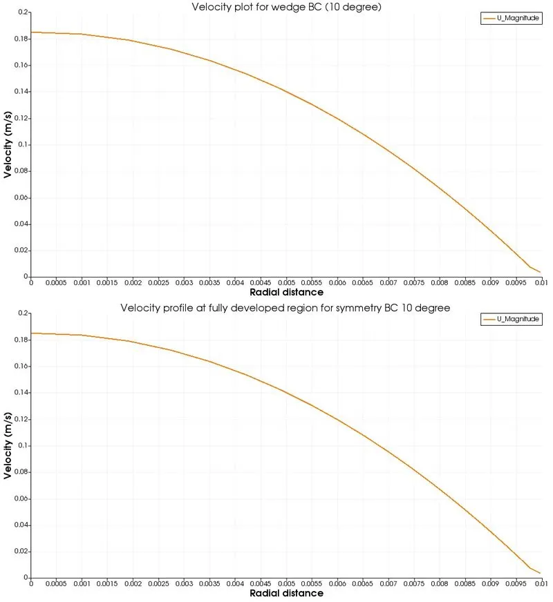
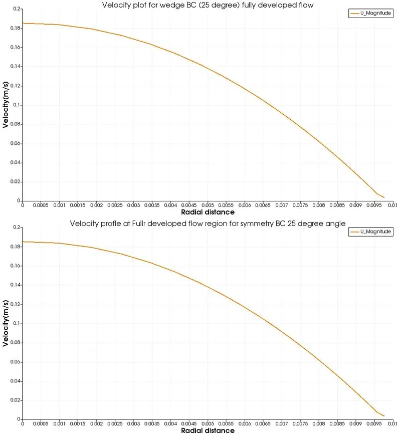
Velocity distribution along the radius at Fully developed flow region
Angle = `10^(circ)`
Angle = `25^(circ)`
Angle = `45^(circ)`
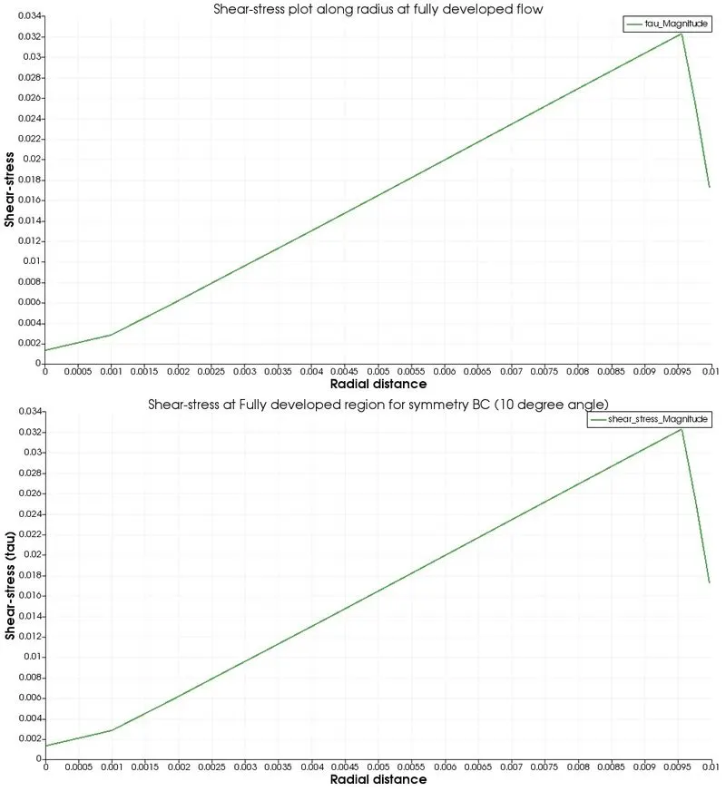
Shear Stress Variation with respect to the Radial Distance
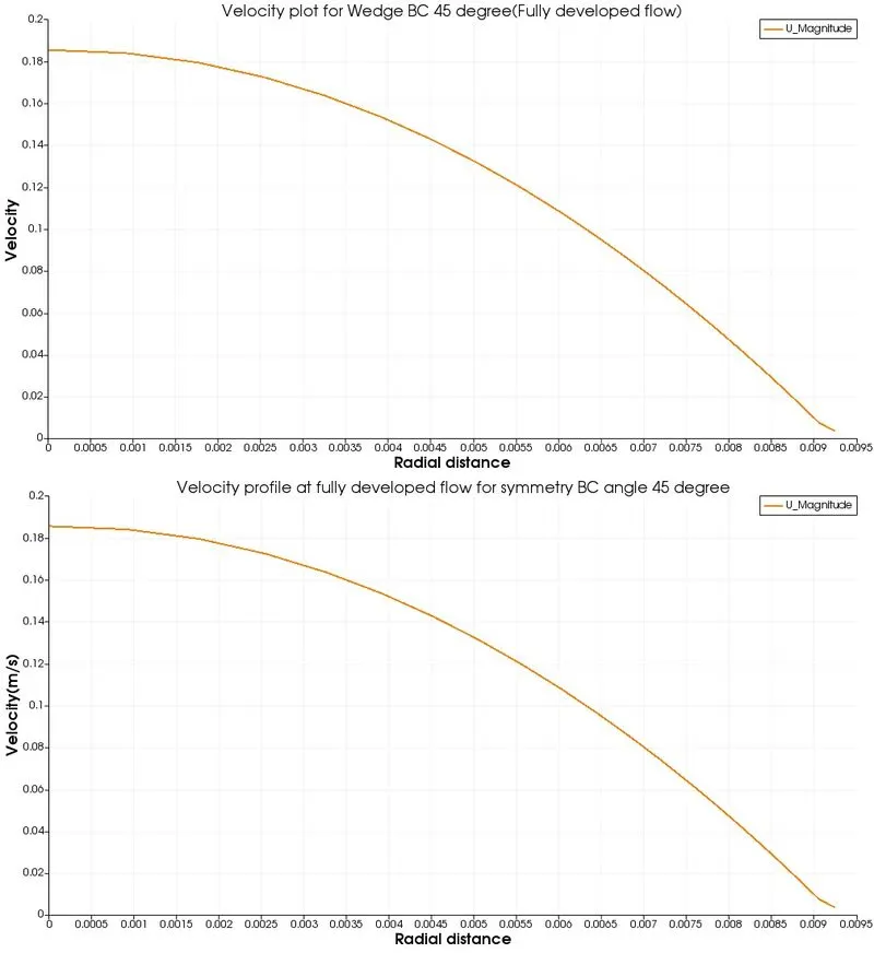
Velocity variation at `10^(circ)`for the two Boundary Conditions (Wedge and Symmetry)
Velocity variation at `25^(circ)` for the two Boundary Conditions.
Velocity variation at `45^(circ)` for the two Boundary Conditions.
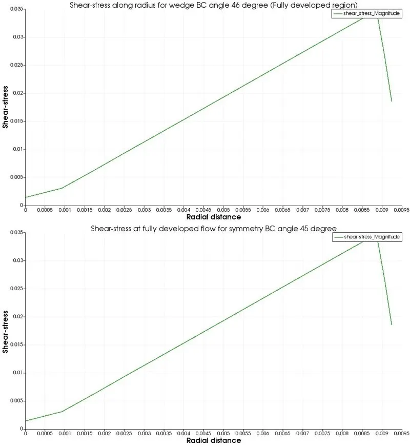
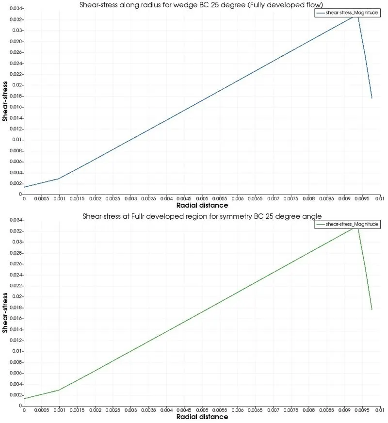
The graph shown above is comparing the Shear Stress for both the boundary conditions for when the wedge angle is `10^(circ), 25^(circ) and 45^(circ)` respectively.
Comparison between two boundary conditions ( Wedge and Synnetry) and also Validation of Numerical results with Analytical results (Hagen-Poiseuille equation)
| Variables | Hagen-poiseuiille | Wedge BC | Wedge BC | Wedge BC | Symmetry BC | Symmetry BC | Symmetry BC |
| equation | (10 degree) | (25 degree) | (45 degree) | (10 degree) | (25 degree) | (45 degree) | |
| Max velocity (m/s) | 0.1878 | 0.1852 | 0.1852 | 0.1852 | 0.1852 | 0.1852 | 0.1852 |
| Wall shear stress (pa) | 0.0335 | 0.0321 | 0.0327 | 0.0327 | 0.0321 | 0.0327 | 0.0327 |
From the above data, it can be concluded that simulation performed for different wedge angles produces similar analytical results.
The deviation from the Hagen-Poiseuille equation is negligible.
Comparison between the two Boundary Conditions
We have performed Simulation for two Boundary Conditions; those are Symmetry Boundary Condition and the Wedge Boundary Condition.
During the Wedge Boundary condition simulation, the simulation across the arc of the wedge is not done, but whereas in the case of Symmetry Boundary Condition, the calculation across the arc of the wedge is done; hence the simulation time is higher in that case. Also, we have observed that the results did not changed due to the change in the Boundary conditions because the Physics of the problem does not change and remains the same.
Conclusions :
- We have simulated the laminar flow through the constant cross-section pipe applying two Boundary Conditions; those are Symmetry Boundary Condition and the Wedge Boundary Condition.
- Simulation has done for the three different wedge angle `10^(circ) , 25^(circ) and 45^(circ)` for all the two boundary conditions.
- We have plotted the velocity profile and shear-stress variations for the above mentioning two different BC at different wedge angle.
- We have observed that the maximum velocity is almost two times of our given initial velocity in inlet.
- Also we have validated our OpenFOAM simulation data with the Hagen-poiseuiille analytical equations.
- From the observation, we can canclude that the simulation performed for different wedge angles produces similar analytical results and the deviation from the Hagen-Poiseuille equation is negligible.