Week 12: Shell and Tube Heat Exchanger simulation

SHELL & TUBE HEAT EXCHANGER SIMULATION:

Aim: To Set up the case for Shell & tubes heat Exchanger and make a comparative study between Parallel Flow and Counter flow simulation using Converge 3.0 CFD program and then post-process the results on Paraview.

Introduction: Shell and tube heat exchangers in their various construction modifications are probably the most widespread and commonly used basic heat exchanger configuration in industry. Shell-and-tube heat exchangers are further classified according to the number of shell and tube passes involved. Shell and tube heat exchangers are typically used for high-pressure applications. This is because the shell and tube heat exchangers can withstand high pressures due to their shape. In this type of heat exchanger, a number of small bore pipes are fitted between two tube plates and primary fluid flows through these tubes. The tube bundle is placed inside a shell and the secondary fluid flows through the shell and over the surface of the tubes.

Shell and tube heat exchangers are, simply put, a device that puts two working fluids in thermal contact using tubes housed within an outer cylindrical shell. These two integral pathways are usually built out of thermally conductive metals that allow easy heat transfer (steel, aluminum alloys, etc.). The tubes carry a fluid from their inlet to their outlet (the “tube-side” flow), while the shell passes a separate fluid over these tubes (the “shell-side” flow). The number of tubes, known as the tube bundle will dictate how much surface area is exposed to the shell-side flow, and therefore determines how much heat is transferred. These devices are among the most effective means of exchanging heat, as they are easily built, maintained, are compact, and provide excellent heat transfer. They are widely distributed in industry, being useful for condensers, turbine coolers, evaporators, feed water preheating, and much more.

Working Principle:

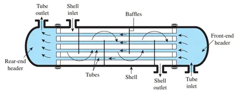
The figure above shows the typical configuration of shell and tube heat exchangers, with labels for easy reading. As previously explained, the fundamental point of shell and tube heat exchangers is to pass a hot fluid through a cold fluid without mixing them, so that only their heat is transferred. The above diagram shows two inlets and two outlets, where each fluid starts at their respective inlet and exits the device at their outlets. The tube-side flow passes through the tube bundle (secured by metal plates known as tubesheets or tubeplates) and exits the tube outlet. Similarly, the shell-side flow starts at the shell inlet, passes over theses tubes, and exits at the shell outlet. The headers on either side of the tube bundle create reservoirs for the tube-side flow and can be split into sections according to specific heat exchanger types.

Baffles: Baffles creates turbulence in the flow of the shell side liquid in a heat exchanger. As turbulence increases it increases the rate of heat transfer. Baffles also provide support to the tubes in a heat exchanger. A little amount of vibration in tubes is acceptable but if the unsupported baffle length is large enough the amplitude of vibration would be equal to spacing between the tubes and this would lead to tube failure because of tubes hitting each other constantly when the liquid flows through the tubes.

There are several reasons for using baffles in heat exchangers, below is a list of functions that baffles are often used for.

• To support tubes in heat exchangers.
• Tubes must be supported at intervals not more than 1.5 m (5 ft), this mainly depends on the diameter of the tube and material of construction. The support intervals can be shorter where flow-induced vibrations occur in certain operations.
• Supporting the tubes using baffles also prevents mechanical vibrations that can result in tubes touching each other and giving rise to leakages and failures mainly near tube sheets
• To enhance heat transfer by directing the flow through the shell in a desired pattern.
• This also increases the turbulence and reduces the stagnant pockets in the heat exchanger. We can also maintain a desired velocity by introducing baffles.

Types of Baffles:

Segmental baffles:

A plate type baffle maybe single segmental, double segmental or triple segmental. With the single and double segmental baffles are most frequently used as they divert the flow most effectively across the tubes.

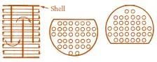Single segmental baffle

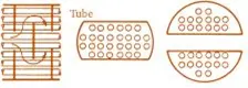Double segmental baffle (Segmental and strip)

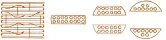Triple segmental baffle

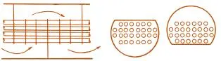No tubes in window segmental baffles

Disk and Doughnut baffles:

Has alternating outer rings and inner disks which directs the flow radially across the tube field. They all very effective in pressure drop to heat transfer conversion.

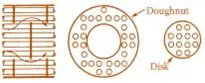Disk and Doughnut baffle

Orifice baffles:

In this type of baffles the shell side fluid follows through the clearance between the tube outside diameter and the baffle hole diameter.

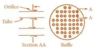Orifice baffle

Rod baffles

This type is metal rods rather than plate metal baffles. The type is use wherever a very low-pressure drop is required. Rod baffles also eliminates the tube vibrations which occur with plate baffles when fluid velocities are high.

The flow in the shell side is mainly parallel to tube axis. Tubes are arranged with square pitch. Rods, with a diameter equal to the clearance between the tube rows, are attached to ring supports and placed between alternate tubes in both horizontal and vertical directions.

The normal rod diameter is 6.35 mm (0.25 inch) and each tube is supported on all four sides at several points along the exchanger. Rod baffles are mainly used when the pressure drop available is very low or there is a pressure drop issue.

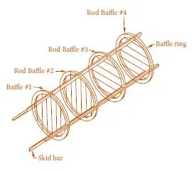Rod baffles

{Data used from - http://www.webbusterz.org/baffles-in-heat-exchangers}

LMTD (Log Mean Temperature Difference):

It is a Logarithmic average of the temperature difference between the hot and cold fluids at each end of the heat exchanger. The larger the LMTD, the more heat is transferred.

Overall Heat Transfer Coefficient (U):

Many of the heat transfer processes encountered in industry involve composite systems and even involve a combination of both conduction and convection. With these composite systems, it is often convenient to work with an overall heat transfer coefficient, known as a U-factor.

Geometry:

- In the Converge Studio first we import the ‘STL’ file of the geometry.

- Then, we carry out a ‘Diagnosis’ on the shape created to check for any errors. If there is no error then the geometry is correct.

- Then we move to case set up.

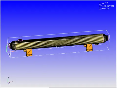
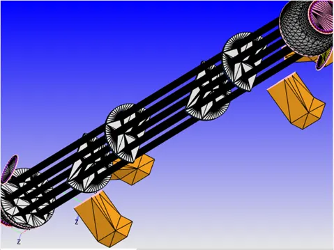
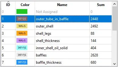
Boundary Flagging:

Boundaries 1 to 7 -

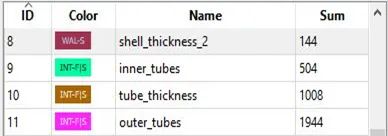
Boundaries 8 to 11 -

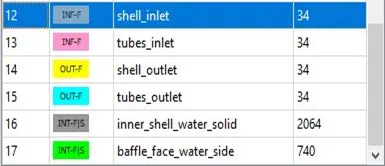
Boundaries 12 to 17 -

Case Set up Procedure:

- Application Type: Time-based

- Material: Select Liquid Simulation, Solid simulation, Species.

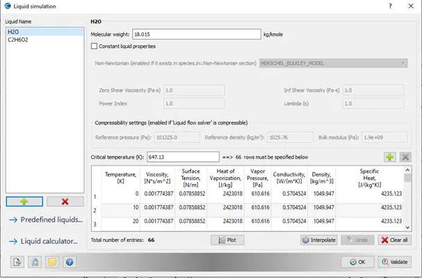
- Liquid Simulation:

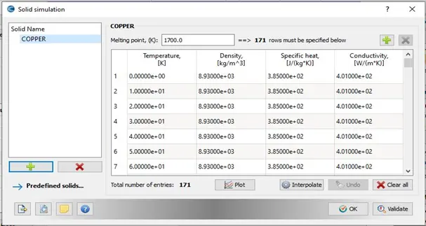
- Solid Simulation:

- Global Transport: Turbulent Prandtl Number = 0.9

Turbulent Schmidt Number = 0.78

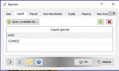
- Species: Liquid Selection as below:

- Species: Solid Selection as below:

- Simulation Parameters:

- Run Parameter: Transient Simulation; Full hydrodynamic mode with Incompressible Liquid Flow Solver.

- Simulation Time Parameter:

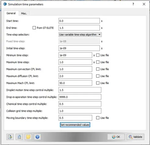
- Solver Parameters:

- Navier-Stokes Solver Type = ‘Density based’ selected.

- Misc.: Strict Conserve = 2-strict conserve for everything including passives.

- Boundary Conditions:

- Boundary Region Defined:

- Outer Tube In Baffles:

- Boundary Type = Interface; Wall motion Type = Stationary

- Forward side Region = Solid 3 Baffle thickness

Boundary Condition - Velocity = Slip; Temperature = Specified Value (DI)

- Reverse side Region = Solid 2 Between Tubes

Boundary Condition - Velocity = Slip; Temperature = Specified Value (DI)

- Outer Shell:

- Boundary Type = Wall; Wall motion Type = Stationary; Surface movement = Fixed

Boundary Condition - Velocity = Slip; Temperature = 300 K

- Shell Legs:

- Boundary Type = Wall; Wall motion Type = Stationary; Surface movement = Fixed

Boundary Condition - Velocity = Slip; Temperature = 300 K

- Shell Thickness:

- Boundary Type = Wall; Wall motion Type = Stationary; Surface movement = Fixed

Boundary Condition - Velocity = Slip; Temperature = 300 K

- Inner Shell Oil Side:

- Boundary Type = Interface; Wall motion Type = Stationary

- Forward side Region = Fluid 1 Oil

Boundary Condition - Velocity = Law of Wall; Temperature = Law of Wall

- Reverse side Region = Solid 1 Between Shells

Boundary Condition - Velocity = Slip; Temperature = Specified Value (DI)

- Baffle:

- Boundary Type = Interface; Wall motion Type = Stationary

- Forward side Region = Fluid 1 Oil

Boundary Condition - Velocity = Law of Wall; Temperature = Law of Wall

- Reverse side Region = Solid 3 Baffle Thickness

Boundary Condition - Velocity = Slip; Temperature = Specified Value (DI)

- Baffle Thickness:

- Boundary Type = Interface; Wall motion Type = Stationary

- Forward side Region = Fluid 1 Oil

Boundary Condition - Velocity = Law of Wall; Temperature = Law of Wall

- Reverse side Region = Solid 3 Baffle Thickness

Boundary Condition - Velocity = Slip; Temperature = Specified Value (DI)

- Shell Thickness 2:

- Boundary Type = Wall; Wall motion Type = Stationary; Surface movement = Fixed

Boundary Condition - Velocity = Slip; Temperature = 300 K

- Inner Tubes:

- Boundary Type = Interface; Wall motion Type = Stationary

- Forward side Region = Fluid 2 Water

Boundary Condition - Velocity = Law of Wall; Temperature = Law of Wall

- Reverse side Region = Solid 2 Between Tubes

Boundary Condition - Velocity = Slip; Temperature = Specified Value (DI)

- Tube Thickness:

- Boundary Type = Interface; Wall motion Type = Stationary

- Forward side Region = Fluid 2 Water

Boundary Condition - Velocity = Law of Wall; Temperature = Law of Wall

- Reverse side Region = Solid 2 Between Tubes

Boundary Condition - Velocity = Slip; Temperature = Specified Value (DI)

- Outer Tubes:

- Boundary Type = Interface; Wall motion Type = Stationary

- Forward side Region = Fluid 1 Oil

Boundary Condition - Velocity = Law of Wall; Temperature = Law of Wall

- Reverse side Region = Solid 2 Between Tubes

Boundary Condition - Velocity = Slip; Temperature = Specified Value (DI)

- Shell Inlet:

- Boundary Type = Inflow;

- Pressure = Zero Normal Gradient (NE)

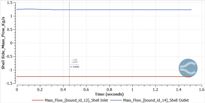
- Velocity (Mass Flow boundary) = 1.252 kg/s;

- Temperature = 348 K

- Species = C₂H₆O₂ (Mass Fraction = 1)

- Tube Inlet:

- Boundary Type = Inflow;

- Pressure = Zero Normal Gradient (NE)

- Velocity (Mass Flow boundary) = 0.037 kg/s;

- Temperature = 300 K

- Species = H₂O (Mass Fraction = 1)

- Shell Outlet:

- Boundary Type = Outflow;

- Pressure = 101325 Pa

- Velocity = Zero Normal Gradient (NE)

- Temperature = 300 K

- Species = C₂H₆O₂ (Mass Fraction = 1)

- Tube Outlet:

- Boundary Type = Outflow;

- Pressure = 101325 Pa

- Velocity = Zero Normal Gradient (NE)

- Temperature = 300 K

- Species = H₂O (Mass Fraction = 1)

- Inner Shell Water Side:

- Boundary Type = Interface; Wall motion Type = Stationary

- Forward side Region = Fluid 2 Water

Boundary Condition - Velocity = Law of Wall; Temperature = Law of Wall

- Reverse side Region = Solid 1 Between Shells

Boundary Condition - Velocity = Slip; Temperature = Specified Value (DI)

- Baffle Face Water Side:

- Boundary Type = Interface; Wall motion Type = Stationary

- Forward side Region = Fluid 2 Water

Boundary Condition - Velocity = Law of Wall; Temperature = Law of Wall

- Reverse side Region = Solid 3 Baffle Thickness

Boundary Condition - Velocity = Slip; Temperature = Specified Value (DI)

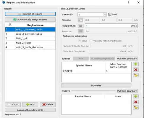
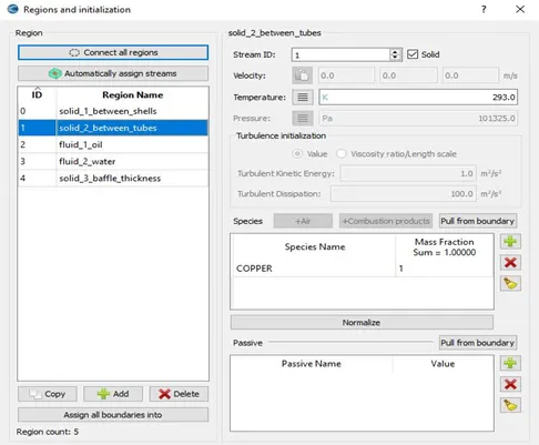
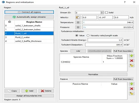
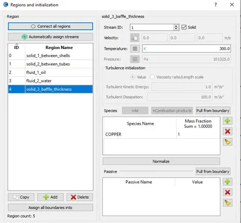
- Initial Conditions & Events: Regions & Initializations:

- Region- 0 [Solid_1_between_shells]: Assigned as Solid region

- Region- 1 [Solid_2_between_tubes]: Assigned as Solid region

- Region- 2 [Fluid_1_oil]: Assigned as Liquid region

- Region- 3 [Fluid_2_water]: Assigned as Liquid region

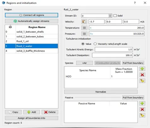
- Region- 4 [Solid_2_between_tubes]: Assigned as Solid region

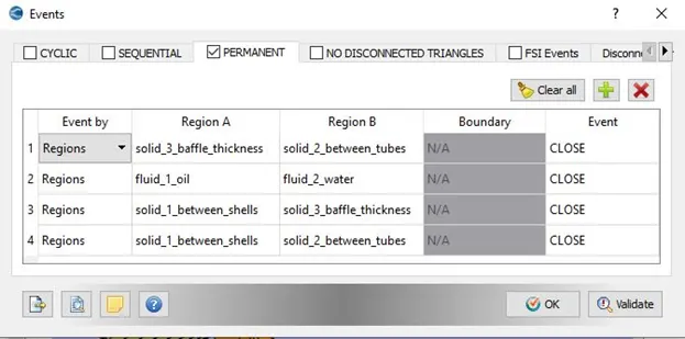
- Events Set-up:

- Physical Models:

- Turbulence Modelling= set to RANS [RNG K-Ɛ]

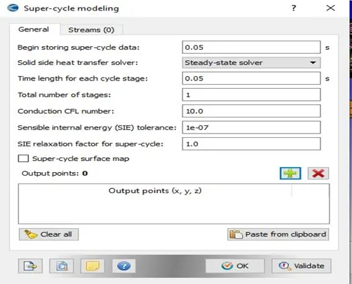
- Super Cycling:

- Grid Control:

Base Grid (in mm): dx = dy = dz = 0.01.

- Post Processing:

- Post variables Selection:

- Typical Variables/Geometry: Select desired variables such as Density, Velocity, pressure, temperature.

- Output Files:

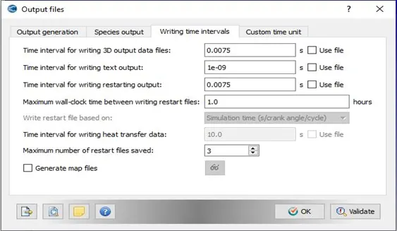
Case setup is complete with this.

- Export case setup: The case setup files are then ‘Exported’ to the destination folders to save the details.

- The destination folders should consist of following files in order to run the simulation and then post process the result on Paraview. The files are:

(i) converge.exe (name changed for the ease of run command on cygwin)

(ii) mpiexec.exe (name changed for the ease of run command on cygwin)

(iii) post_convert.exe (under output folder)

- Open Cygwin: Now the simulation is run using Cygwin. We navigate to the desired folder where the setup files were exported.

- Command to Run Simulation: The command to run simulation through Cygwin for Converge Studio 3.0 version is as below:

“ mpiexec.exe –n 2 converge.exe restricted “

• The simulation starts running, due to which output files are generated under a separate output folder.
• These output files are then post processed to convert the data in a format suitable for Paraview.

- Inline Plot: In the Converge Studio program, we can use Inline Plotting option to plot the curves during simulation run. We can observe the change in the plots and see the simulation reach the steady state condition at the end of the plot.

- Post Convert in Converge: To post process, we use file type as ‘Paraview VTK in-line binary format’. Now the files are post processed with a case name ‘test’.

• This generates ‘test.vtm’ group files which are generally used in Paraview to observe the results.

- Paraview: Open Paraview to check for the results.

(A) Observations for Parallel Flow:

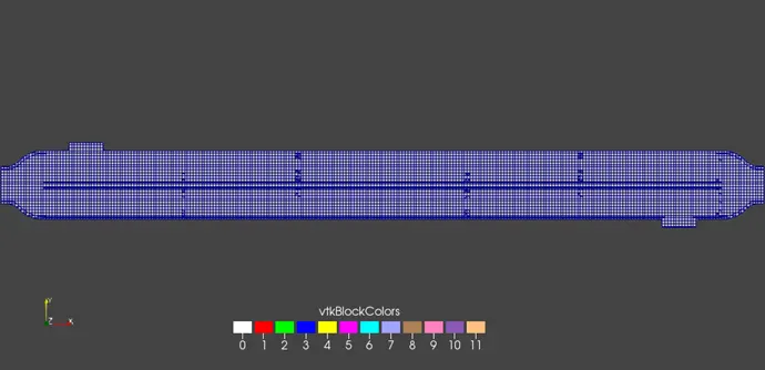
Mesh Formation:

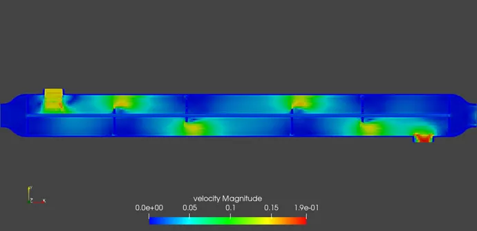
Velocity Contour:

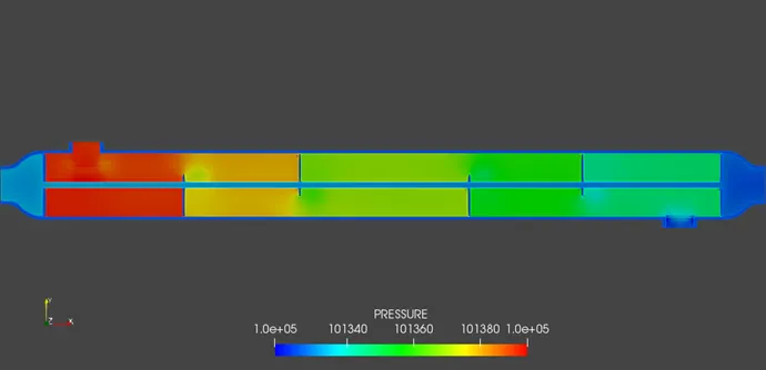
Pressure Contour:

Temperature Contour:

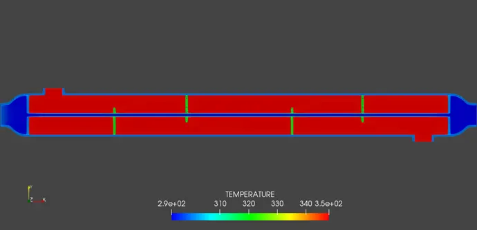
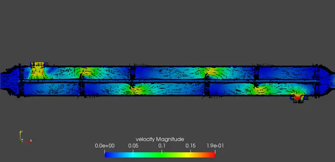
Glyph Contour:

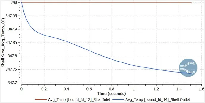
Temperature Plot – Shell Side:

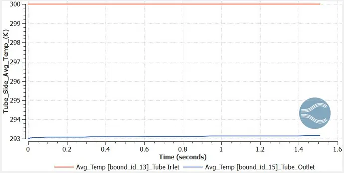
Temperature Plot – Tube Side:

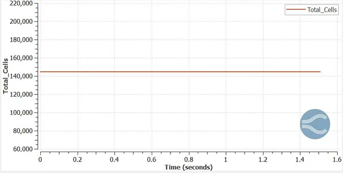
Total Cell Count:

Mass Flow Rate Shell side:

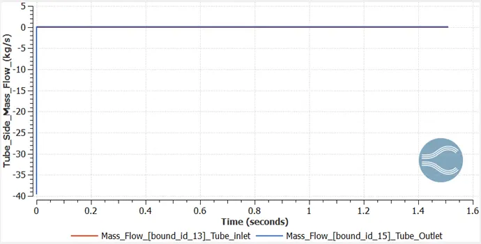
Mass Flow Rate Tube side:

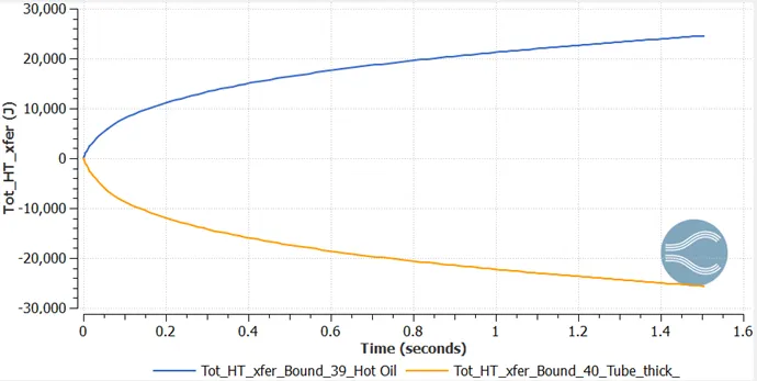
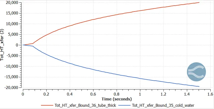
Total Heat Transfer between Hot Oil & Tube:

Total Heat Transfer between Tube & Cold Water:

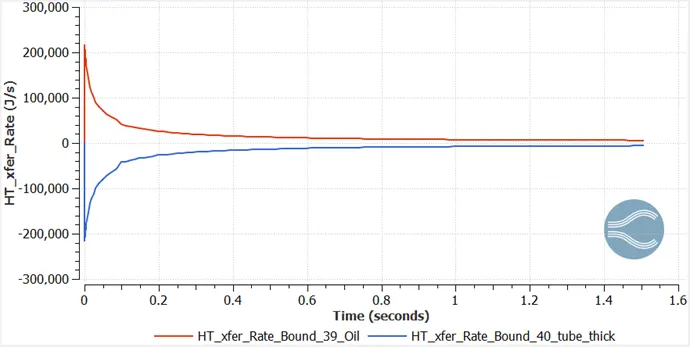
Heat Transfer Rate between Hot Oil & Tube:

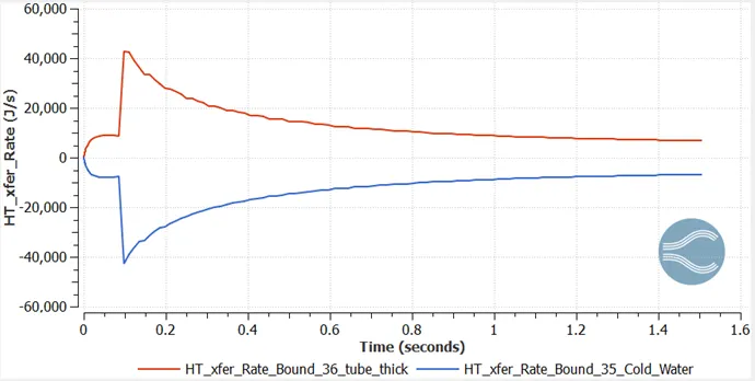
Heat Transfer Rate between Tube & Cold Water:

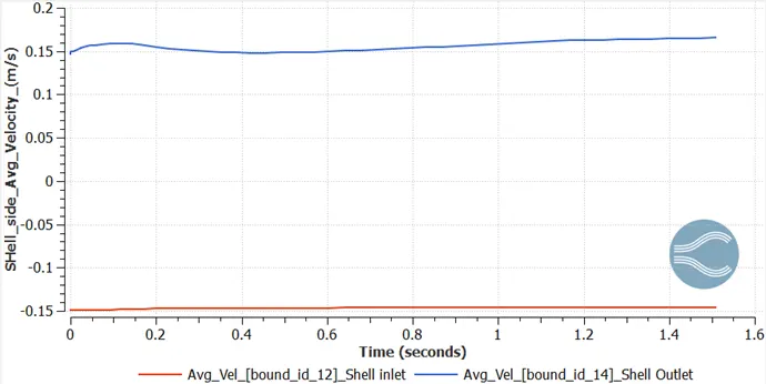
Velocity Plot – Shell Side:

Velocity Plot – Tube Side:

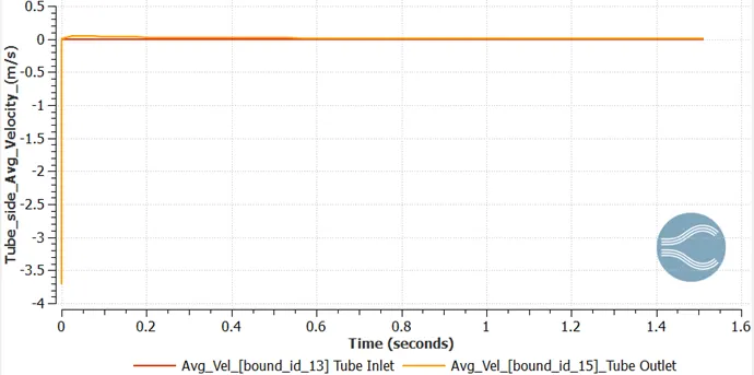
Velocity Animation: https://youtu.be/OKA-0itiSbw

Pressure Animation: https://youtu.be/g2h4m8P5Qos

Calculations for Parallel Flow:

• LMTD calculations:

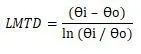
Here –

Ɵ_i = T_hi - T_co = 75°C – 20°C = 55°C

Ɵ_o = T_ho - T_ci = 74.7°C – 27°C = 47.7°C

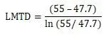
LMTD = 51.26°C

(B) Heat Loss in Heat Exchanger:

From the plots of Counter Flow process, we get the following results to calculate the heat loss-

Heat released by Hot Oil = 24537 J

Heat released by Cold Water = 19548 J

Thus, Heat absorbed by solid (tube material) = 24537 – 19548 = 4989 J

So, in order to reduce the heat loss to the solid and obtain better heat transfer between hot and cold fluid, the selection optimum material for solid is crucial.

The heat loss can be reduced by selecting a material with ‘High Conductivity’.

(C) Heat Transfer Rate Calculations:

Calculations mentioned below are for Hot Oil-

Q = ṁ x C_p x ΔT

Here-

ṁ = 1.252 Kg/s

C_p = 2600 J/kgK

ΔT = 75°C - 74.7°C = 0.3°C

Therefore,

Q = 1.252 x 2600 x 0.3 = 976.56 J/s = 976.56 W

(D) Overall Heat Transfer Coefficient Calculations:

Q = U x A x LMTD

Here-

A (Area) = π x d_o x L x n

= 3.14 x 0.023 x 2.4 x 7

= 1.2133 m²

LMTD = 51.28°C

Therefore,

976.56 = U x 1.2133 x 51.28

U = 15.69 W/m²K

(B) Observations for Counter Flow:

Velocity Contour:

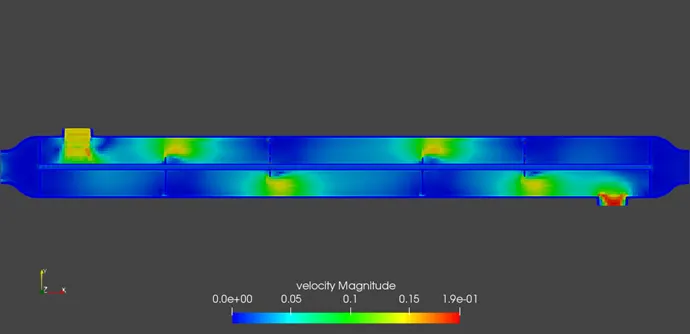
Pressure Contour:

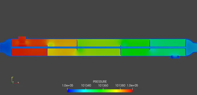
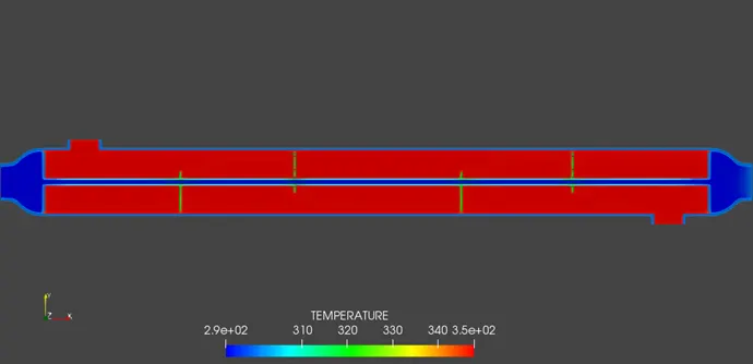
Temperature Contour:

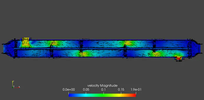
Glyph Contour:

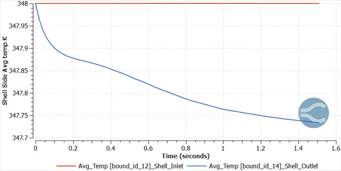
Temperature Plot – Shell Side:

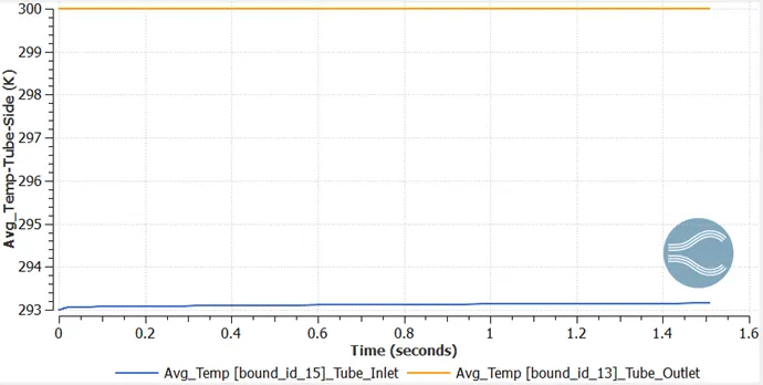
Temperature Plot – Tube Side:

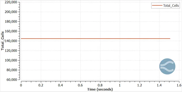
Total Cell Count:

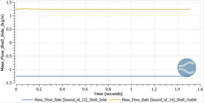
Mass Flow Rate Shell side:

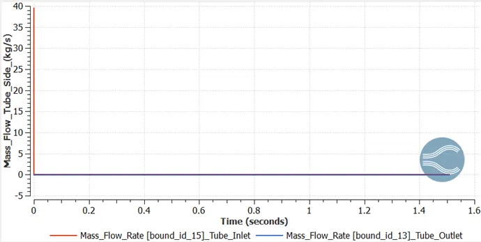
Mass Flow Rate Tube side:

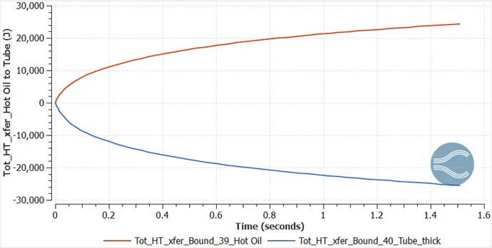
Total Heat Transfer between Hot Oil & Tube:

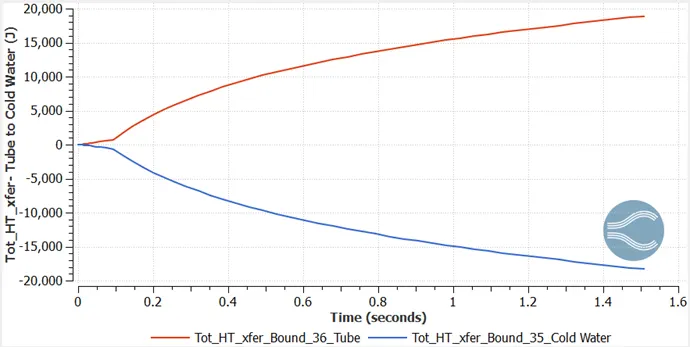
Total Heat Transfer between Tube & Cold Water:

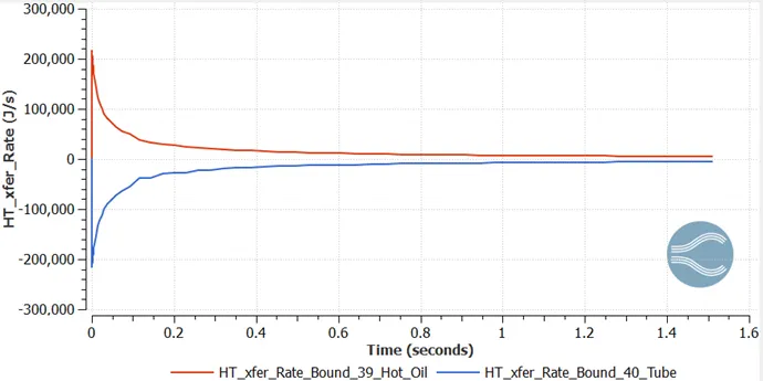
Heat Transfer Rate between Hot Oil & Tube:

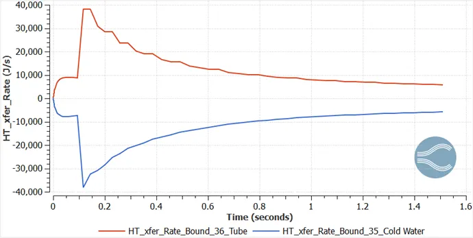
Heat Transfer Rate between Tube & Cold Water:

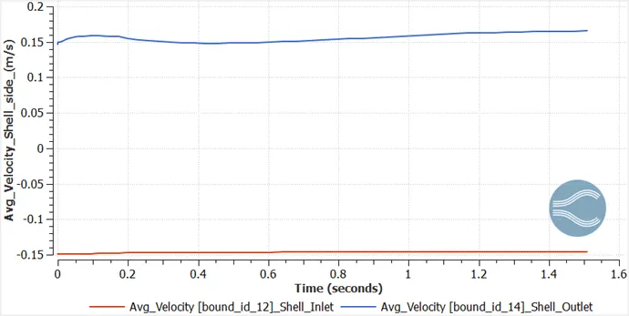
Velocity Plot – Shell Side:

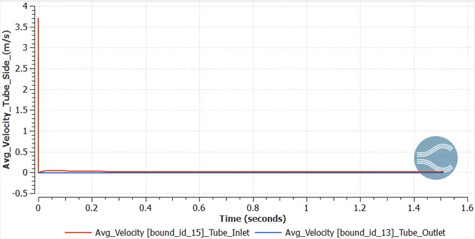
Velocity Plot – Tube Side:

Velocity Animation: https://youtu.be/E19PHFO7ymc

Pressure Animation: https://youtu.be/ryDisSKS8AQ

Calculations for Counter Flow:

• LMTD calculations:

Here –

Ɵ_i = T_hi - T_co = 75°C – 27°C = 48°C

Ɵ_o = T_ho - T_ci = 74.7°C – 20°C = 54.7°C

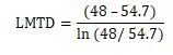
LMTD = 51.28°C

(B) Heat Loss in Heat Exchanger:

From the plots of Counter Flow process, we get the following results to calculate the heat loss-

Heat released by Hot Oil = 24313 J

Heat released by Cold Water = 18301 J

Thus, Heat absorbed by solid (tube material) = 24313 – 18301 = 6012 J

So, in order to reduce the heat loss to the solid and obtain better heat transfer between hot and cold fluid, the selection optimum material for solid is crucial.

The heat loss can be reduced by selecting a material with ‘High Conductivity’.

(C) Heat Transfer Rate Calculations:

Calculations mentioned below are for Hot Oil-

Q = ṁ x C_p x ΔT

Here-

ṁ = 1.252 Kg/s

C_p = 2600 J/kgK

ΔT = 75°C - 74.7°C = 0.3°C

Therefore,

Q = 1.252 x 2600 x 0.3 = 976.56 J/s = 976.56 W

(D) Overall Heat Transfer Coefficient Calculations:

Q = U x A x LMTD

Here-

A (Area) = π x d_o x L x n

= 3.14 x 0.023 x 2.4 x 7

= 1.2133 m²

LMTD = 51.28°C

Therefore,

976.56 = U x 1.2133 x 51.28

U = 15.69 W/m²K

Comparison: For a similar operating conditions Counter Flow heat exchangers and efficient than parallel flow heat exchangers. The counter flow heat exchangers need less space than parallel flow due to higher efficiency. This distributes the heat more evenly across the heat exchanger and allows for maximum efficiency.

Drawbacks of Shell and Tube Heat Exchangers:

• It requires more space than other type of heat exchangers for similar applications such as plate heat exchangers.
• Maintenance and cleaning is a tedious process which consumes a lot of time and needs longer plant shut down time.
• Once designed and manufactured, the capacity of these heat exchangers cannot be increased as against plate heat exchangers wherein plates can be increased thus increasing its capacity.
• Due to the above reasons their effectiveness in various applications reduces.

Fouling & its effects: Due to continuous usage and the surface of heat exchanger is not cleaned at a regular interval then scaling occurs. This phenomenon called fouling in a heat exchanger. Fouling reduces the heat transfer coefficient and thus reducing its efficiency. So, while designing a shell & tube heat exchanger fouling margins need to be taken into account.

Results:

1. Simulation Time for Parallel Flow = 1604 seconds
2. Simulation time for Counter Flow = 1838 seconds

Conclusion:

We can conclude from the simulation using Converge CFD program, that with finer mesh sizes the results obtained become prominent and accurate. The change in the parameters for a flow can be observed from the various animations, plots, contours and profiles and understand how the results reach steady state.