Week 12- Major Project (CFD Analysis on Combustion in a SCRAMJET engine)

AIM: To calculate the most efficient slot-fuel injector and cavity-flame holder for a scramjet in ANSYS Fluent.

THEORY:

• A scramjet engine is an improvement over the traditional ramjet engine as it efficiently operates at hypersonic speeds and allows supersonic combustion. Thus it is known as Supersonic Combustion Ramjet or Scramjet. The engine uses the velocity of supersonic flow to compress the incoming air.

This is the schematic diagram:

 

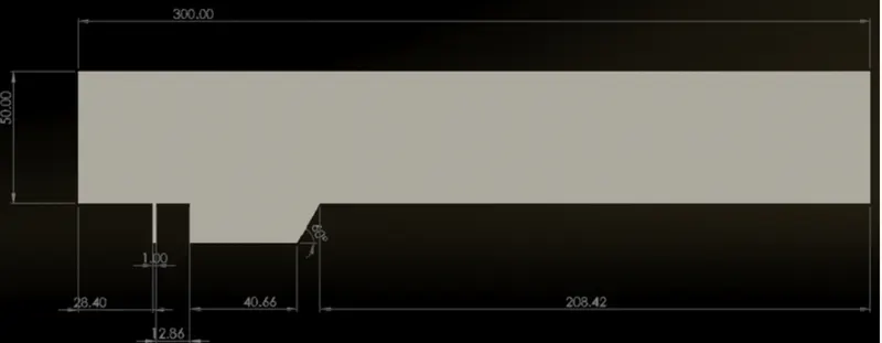
• A fuel slot is a small tube attached to the tube of the main engine, which serves as the inlet for fuel.

• The angle visible is called the fuel-injector angle, this angle will be varied through the simulation and the results of the angle will be seen.

• A cavity is an extension from the tube of the main engine and serves as a side-stop for combustion so that the main airflow isn't affected.

• The angle visible is called the angle of the cavity. This angle will be varied throughout this simulation, and its effects will be seen.

• The fuel used in this simulation is Hydrogen and the combustion reaction is as follows:

  2H2(g)+O2(g)→2H2O(g)+energy">2H2(g)+O2(g)→2H2O(g)+energy

Combustion Efficiency:

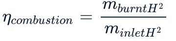
• It is defined as the ratio of burnt fuel to the total fuel for an engine.
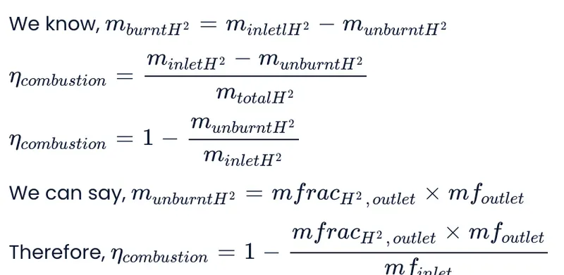
• In this case, its case the efficiency can be said as: 

• The project is divided into three cases, each case is further divided into a number of sub-cases. In each case, the Combustion Efficiency will be calculated.

Case 1: The fuel-injector angle is fixed at 90 degrees, while the angle of the cavity is set to 30, 45 and 60 degrees.

Case 2: The angle of the cavity is set to 60 degrees, while the fuel-injector angle is set to 20, 30, 45, 60 and 90 degrees.

Case 3: The fuel-injector is placed inside the cavity, for different angles of cavity and fuel-injector angles.

• Finding the combustion efficiency for 15 cases is infeasible and the goal of the project is to find the most efficient configuration for the engine. The angles for case 3 will be chosen on the basis of the results from Case 1 and Case 2.

GEOMETRY:

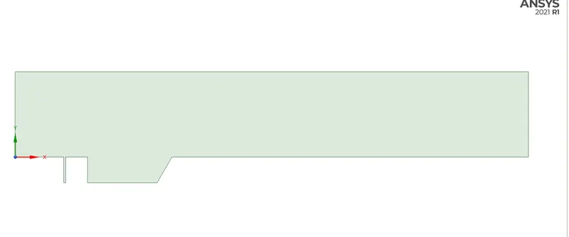
• The geometry is a sketch created in SpaceClaim with the appropriate angles of cavity and fuel-injector, this geometry is converted into a surface using the pull tool. Named selections are defined for all the boundaries. This is the final geometry for a case:

MESHING:

• The default quadrilateral mesh is used for all simulations. Capture Proximity is turned on to ensure the region near the fuel injector is more refined.

  This is the Mesh before exporting to Fluent:

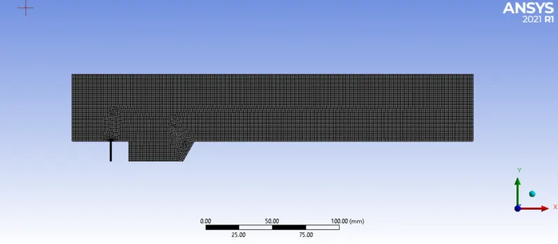
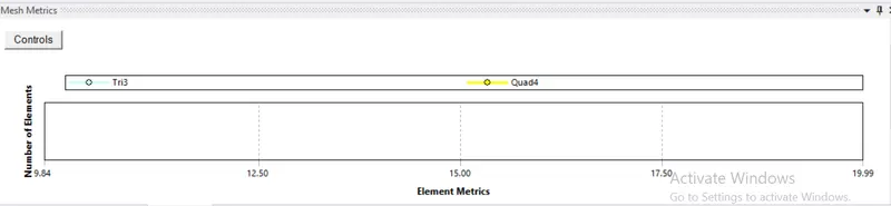
• As the quality of most elements is greater than 0.9, this mesh can be said to be of satisfactory quality.

• The mesh roughly contains 16257 nodes and 15847 elements, and this number will vary for each case.

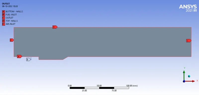
• And its named selections,

SIMULATION SETUP:

General:

• The simulations used a pressure-based, 2D, steady-state solver.

Materials:

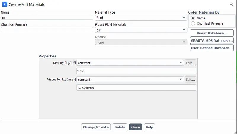
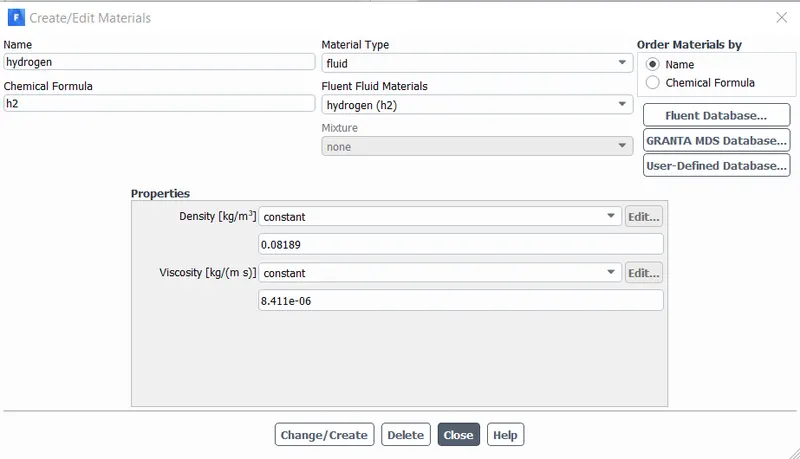
• Air and Hydrogen gas (fluid) was used for this simulation.
• The properties were the default ones as shown below,

Hydrogen,

Turbulence Model:

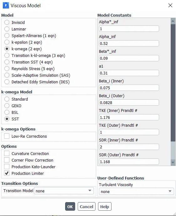
• While doing a literature review for this project, the two most commonly used models were: k-omega SST and k-epsilon. In the end, the model chosen was k-omega SST due to its flexibility in capturing boundary layers for any y+/velocity. [1]

Species:

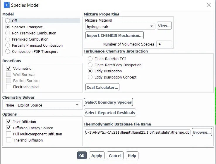
This introduces 2 more materials, they are: O2 and H2O

Boundary Conditions:

• inlet-air - velocity-inlet, 1040 m/s velocity, 600K temperature, and O2 with a mole fraction of 0.21 (to simulate atmospheric air).
• inlet-fuel - velocity-inlet, 200 m/s velocities, 500 bar pressure (5×107Pa), and H2O with a mole fraction of 1 (pure hydrogen).
• outlet - pressure-outlet, 0Pa.
• walls-bottom, walls-top - stationary wall.
• Boundary Conditions were decided after an extensive literature review and were chosen from Reference [1]

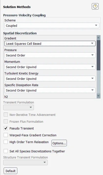
Solution Methods:

Reports:

Three reports were generated for each iteration, they are:

• outlet-mass-flow - this report generates the mass flow rate at the outlet.
• mass-flow-rate-inlet-fuel - this report generates the mass flow rate of the fuel at the inlet.
• mf-h2-outlet - this generates the mass fraction of fuel at the outlet.

Combustion Efficiency:

To calculate the combustion efficiency using the following formula:

CFD Setup

All Simulations were conducted using Ansys Fluent 22 R2. The fluid used in the domain was the predefined hydrogen-air mixture for the global step combustion mechanism. The density of the individual species was estimated using the ideal gas formulation. The air and fuel inlets were set to a pressure inlet with a pressure outlet at the rear. The operating conditions were set to 0Pa. The injection fuel injection angle was varied for the respective simulation using components.

The detailed boundary conditions were derived from the works of Wang et al[2] and can be seen in the table below.

Parameter	Inlet Air	Inlet Fuel
Mach	2.52	1.0
Total Pressure	1.6 MPa	0.8 MPa
Total Temperature	1486	300
Mass Fraction O2">O2	0.2338	0
Mass Fraction H2O">H2O	0.0622	0
Mass Fraction N2">N2	0.7040	0
Mass Fraction H2">H2	0	1

Using the above boundary conditions resulted in the equivalence ratio of the combustion: ϕ">ϕ= 0.62. 

The steady-state pressure-based PV-coupled solver was used for the spatial discretization of the flow parameters. The energy equation was enabled for the simulation. Turbulence was estimated using the two-equation K-Omega SST turbulence model. The volumetric reaction kinetics was modeled using the finite-rate/eddy-dissipation model. The second-order scheme was used to estimate the pressure, the second-order upwind scheme was used to estimate momentum, energy, species, and turbulence parameters. The solution was initialized using standard initialization followed by an FMG initialization to quicken the simulation runtime. The pseudo-transient method was also used with an automatic conservative length scale. 

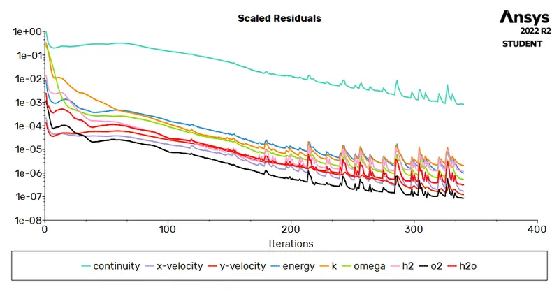
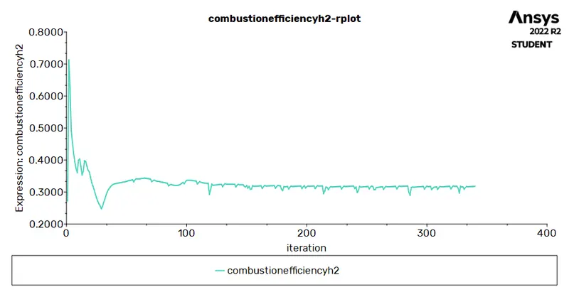
Convergence was monitored using the scaled residuals and the variations of combustion efficiency across iterations. The simulations were assumed to be converged when the combustion efficiency varied under 0.001 across 10 iterations and scaled residuals were all below 1e-3. The simulation typically ran for 300 iterations to achieve convergence.

Results

The typical convergence of the scaled residuals and the combustion efficiency can be seen in the images below. 

The results of the combustion efficiency for the various cases can be seen in the table below. 

Case no.	Wedge Angle	Injection Angle	Injector Position	Combustion Efficiency %
1	30	90	Before Cavity	21.28
2	45	90	Before Cavity	21.68
3	60	90	Before Cavity	22.23
4	60	60	Before Cavity	26.17
5	60	45	Before Cavity	28.01
6	60	30	Before Cavity	33.47
7	60	20	Before Cavity	36.40
8	30	90	At Cavity	31.80
9	45	90	At Cavity	31.20
10	60	90	At Cavity	29.94
11	60	60	At Cavity	47.57
12	60	45	At Cavity	62.83
13	60	30	At Cavity	78.44
14	60	20	At Cavity	62.44

From the above table, case 13 with a fuel injection angle of 30 degrees, 60 degrees wedge angle, and in-cavity fuel injector has the highest combustion efficiency of 78.44%. A steady increase in combustion efficiency can also be seen in decreasing fuel injection angles. When the injection angle is maintained at a const 90 degrees, increasing the wedge angle is shown to increase the combustion efficiency in cases where the injector is before the cavity, but decreases combustion efficiency when the injector is placed at the cavity. Overall, the placement of the injector inside the cavity shows higher combustion efficiency in all cases compared to the corresponding cases of the injector placed before the cavity.

The images below show the Mach no distribution from case 13 (top) with the best combustion efficiency and case 1 (bottom) with the lowest combustion efficiency. 

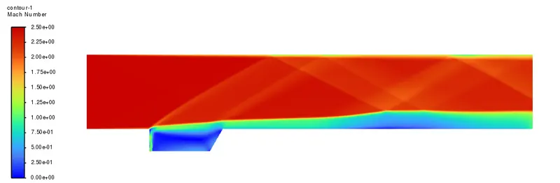
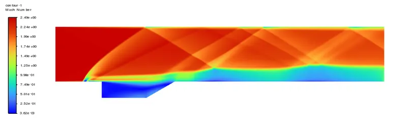
Oblique shocks can be seen emanating from the shear layer in both cases reflecting between the upper walls and the shear layer. Case 1 has more oblique shocks and reflections compared to case 13 and can be attributed to the fuel injection flowing transverse into the free stream supersonic flow creating a large obstruction to the flow. 

The images below show the static temperature distribution from case 13 (top) with the best combustion efficiency and case 1 (bottom) with the lowest combustion efficiency. 

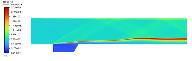
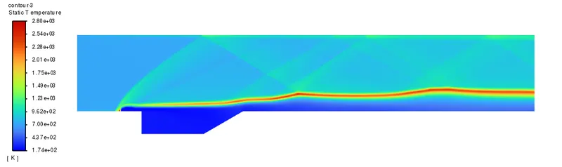
The highest temperature can be seen in case 1 to be 2800K while case 13 reaches a maximum temperature of 2330K. These rises in temperatures strongly indicate the occurrence of supersonic combustion in the supersonic flow. 

The images below show the mass fractions distribution of H2 and H2O from case 13 (top) with the best combustion efficiency and case 1 (bottom) with the lowest combustion efficiency. 

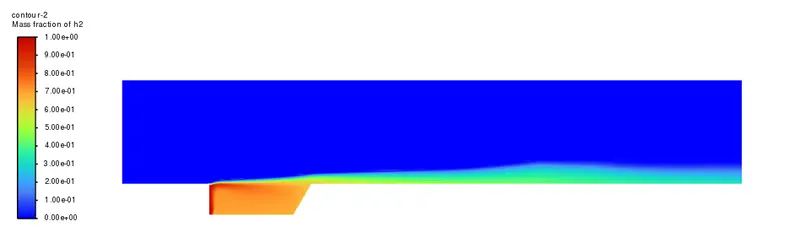
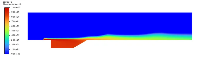
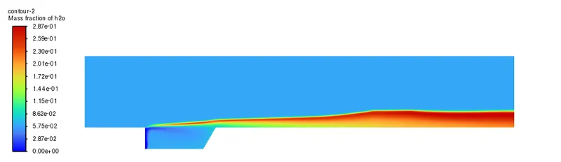
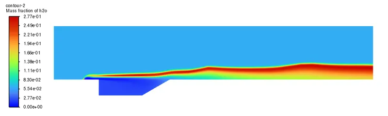
A steady decline in the mass fraction of H2 and an increase in the mass fraction of H2O can be seen downstream of the cavity in both cases. The traces of unburnt H2 at the outlet is seen to be more in case 1 compared to case 13 and this directly leads to the difference in combustion efficiency. A similar trend is seen for the mass fraction of H2O at the outlet as well. 

Conclusion

Simulation of supersonic combustion was conducted using the given cavity-based combustor geometry with varying wedge angle, fuel injection angle, and fuel injector positions. The combustion efficiencies of all the cases were compared to arrive at the best configuration. The combustor configuration with a 60 degrees wedge angle, 30 degrees fuel injection, and the injector placed inside the cavity showed the highest combustion efficiency of 78.44%.