Week 11 - Simulation of Flow through a pipe in OpenFoam
Simulation of Flow through a pipe in OpenFoam
Objective:
The aim of this project is to simulate the flow of water through a pipe and validate the results of the fully developed flow with analytical solutions.
Introduction:
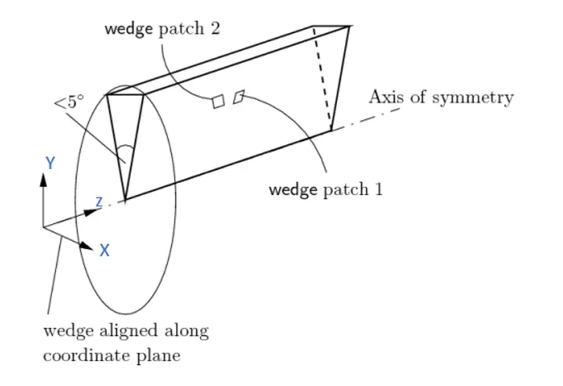
The internal flow through the pipe is an axisymmetric problem. Hence the simulation is simplified to a wedge geometry as shown in the figure
Hydrodynamic length is the length the fluid must travel inside a pipe before it becomes fully developed. Normally, the fluid would enter the pipe with uniform velocity. As the surface of the pipe is stationary, the layer of the fluid coming in contact with the pipe surface also becomes stationary due to the no-slip condition. The viscous forces within the fluid resist the adjacent layers leading to the development of a velocity profile with high velocity at the centre of the pipe [1]. This phenomenon is illustrated in the figure below:
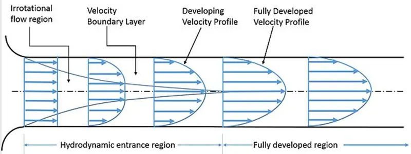
The entrance length depends on the velocity of the fluid, its density and viscosity. For a laminar flow, it can be calculated using the following equation :
L_(h , laminar)=0.05* 〖Re〗_D* D
Where 〖Re〗_D= (ρ * v * D)/μ
D – diameter of the pipe
– density of fluid
µ - dynamic viscosity of the fluid
v – velocity of fluid
Hagen-Poiseuille Equation:
The Hagen-Poiseuille equation is used to determine the pressure loss in a steady, hydrodynamically fully-developed, no-swirl flow in a circular pipe. It is given as follows
∆p= (8* μ* V_(avrg )* L)/R^2
Where
µ is the dynamic viscosity
is the average velocity
L is the length of the pipe
R is the radius of the pipe
Input data and parameters:
Diameter of the pipe D = 0.003 meters
Radius r = D/2 meters
Reynold’s Number Re = 2100
Hydrodynamic entry length Le = 0.05*Re*D
Total length of pipe L = 0.35 + Le
Angle of wedge = 3°
Density of water = 997 Kg /m^3
Dynamic viscosity µ = 0.000890 N*s/m^2
Kinematic viscosity v = µ/ρ
Average velocity V_avg= (R_e* μ)/(ρ*D)
Maximum velocity u_(max )=2* V_avg
Kinematic pressure k_p= ∆p/ρ
MATLAB CODE :
clear all
close all
clc

% Input Data (meters)
D = 0.003;                 % Diameter
r = D/2;                   % Radius
Re = 2100;                 % Reynolds Number
L_e = 0.05*Re*D;           % Hydrodynamic Entry length
L = 0.35 + L_e;            % Total Length
theta = 3;                 % Wedge Angle

scale = 1;                 % All values referenced to 1 meter scale

% Vertices
v0 = [0 0 0];
v1 = [0 r*cosd(theta/2) r*sind(theta/2)];
v2 = [0 r*cosd(theta/2) -r*sind(theta/2)];
v3 = [L 0 0];
v4 = [L r*cosd(theta/2) r*sind(theta/2)];
v5 = [L r*cosd(theta/2) -r*sind(theta/2)];

% Block Parameters
pointx = 50; % Cells along x-axis
Pointy = 1; % Cells along y-axis
Pointz = 100; % Cells along z-axis
gradx = 1; % Grading along x-axis
grady = 1; % Grading along y-axis
gradz = 1; % Grading along z-axis

% Arc inputs
arc1 = [1,2];
arc2 = [4,5];

f1 = fopen('BlockMeshDict.txt','w');
fprintf(f1,'%s\n','/*--------------------------------*- C++ -*----------------------------------*')
fprintf(f1,'%s\n','  =========                 |')
fprintf(f1,'%s\n','  \      /  F ield         | OpenFOAM: The Open Source CFD Toolbox')
fprintf(f1,'%s\n','   \    /   O peration     | Website:  https://openfoam.org')
fprintf(f1,'%s\n','    \  /    A nd           | Version:  6')
fprintf(f1,'%s\n','     \/     M anipulation  |')
fprintf(f1,'%s\n','*---------------------------------------------------------------------------*/')
fprintf(f1,'%s\n','FoamFile')
fprintf(f1,'%s\n','{')
fprintf(f1,'%s\n','      format        ascii;')
fprintf(f1,'%s\n','      class         dictionary;')
fprintf(f1,'%s\n','      object        blockMeshDict;')
fprintf(f1,'%s\n','}');
fprintf(f1,'%s\n','// * * * * * * * * * * * * * * * * * * * * * * * * * * * * * * * * * * * * * //');
fprintf(f1,'%s %d;\n','convertToMeters',scale);

% Defining Vertices
fprintf(f1,'\t \n')
fprintf(f1,'%s\n','vertices')
fprintf(f1,'%s\n','(')
fprintf(f1,'\t (%d %d %d) \n',v0(1),v0(2),v0(3))
fprintf(f1,'\t (%d %d %d) \n',v1(1),v1(2),v1(3))
fprintf(f1,'\t (%d %d %d) \n',v2(1),v2(2),v2(3))
fprintf(f1,'\t (%d %d %d) \n',v3(1),v3(2),v3(3));
fprintf(f1,'\t (%d %d %d) \n',v4(1),v4(2),v4(3));
fprintf(f1,'\t (%d %d %d) \n',v5(1),v5(2),v5(3));
fprintf(f1,'%s\n',');');

% Defining Blocks
fprintf(f1,'\t \n')
fprintf(f1,'%s\n','blocks')
fprintf(f1,'%s\n','(')
fprintf(f1,'\t hex (0 1 2 0 3 4 5 3) (%d %d %d) %s (%d %d %d)\n',pointx,Pointy,Pointz,'simpleGrading',gradx,grady,gradz)
fprintf(f1,'%s\n',');');

% Defining Edges
fprintf(f1,'\t \n')
fprintf(f1,'%s\n','edges')
fprintf(f1,'%s\n','(')
fprintf(f1,'\t arc %d %d (%d %d %d) \n',arc1(1),arc1(2),0,r,0);
fprintf(f1,'\t arc %d %d (%d %d %d) \n',arc2(1),arc2(2),L,r,0);
fprintf(f1,'%s\n',');');

% Defining Boundaries
fprintf(f1,'\t \n')
fprintf(f1,'%s\n','boundary')
fprintf(f1,'%s\n','(')
fprintf(f1,'\t inlet \n \t { \n')
fprintf(f1,'\t\t type patch; \n')
fprintf(f1,'\t\t faces \n \t\t ( \n')
fprintf(f1,'\t\t\t (0 1 2 0) \n')
fprintf(f1,'\t\t ); \n \t } \n')

fprintf(f1,'\t outlet \n \t { \n')
fprintf(f1,'\t\t type patch; \n')
fprintf(f1,'\t\t faces \n \t\t ( \n')
fprintf(f1,'\t\t\t (3 4 5 3) \n')
fprintf(f1,'\t\t ); \n \t } \n')

fprintf(f1,'\t front \n \t { \n')
fprintf(f1,'\t\t type wedge; \n')
fprintf(f1,'\t\t faces \n \t\t ( \n')
fprintf(f1,'\t\t\t (0 3 4 1) \n')
fprintf(f1,'\t\t ); \n \t } \n')

fprintf(f1,'\t back \n \t { \n')
fprintf(f1,'\t\t type wedge; \n')
fprintf(f1,'\t\t faces \n \t\t ( \n')
fprintf(f1,'\t\t\t (0 3 5 2) \n')
fprintf(f1,'\t\t ); \n \t } \n')

fprintf(f1,'\t top \n \t { \n')
fprintf(f1,'\t\t type wall; \n')
fprintf(f1,'\t\t faces \n \t\t ( \n')
fprintf(f1,'\t\t\t (1 2 5 4) \n')
fprintf(f1,'\t\t ); \n \t } \n')

fprintf(f1,'\t axis \n \t { \n')
fprintf(f1,'\t\t type empty; \n')
fprintf(f1,'\t\t faces \n \t\t ( \n')
fprintf(f1,'\t\t\t (0 3 3 0) \n')
fprintf(f1,'\t\t ); \n \t } \n')
fprintf(f1,'); \n')
fprintf(f1,'\t \n')
fprintf(f1,'%s\n','mergePatchPairsn \n ( \n ); \n')
fprintf(f1,'\t \n')
fprintf(f1,'// ************************************************************************* //')
fclose(f1)
BlockMeshDict :
/*--------------------------------*- C++ -*----------------------------------*\
  =========                 |
  \\      /  F ield         | OpenFOAM: The Open Source CFD Toolbox
   \\    /   O peration     | Website:  https://openfoam.org
    \\  /    A nd           | Version:  10
     \\/     M anipulation  |
\*---------------------------------------------------------------------------*/
FoamFile
{
    format      ascii;
    class       dictionary;
    object      blockMeshDict;
}
// * * * * * * * * * * * * * * * * * * * * * * * * * * * * * * * * * * * * * //

convertToMeters 1;

vertices
(
	 (0 0 0)
	 (0 1.499486e-03 3.926542e-05)
	 (0 1.499486e-03 -3.926542e-05)
	 (6.650000e-01 0 0)
	 (6.650000e-01 1.499486e-03 3.926542e-05)
	 (6.650000e-01 1.499486e-03 -3.926542e-05)
);

blocks
(
	 hex (3 4 5 3 0 1 2 0) (50 1 100) simpleGrading (1 1 1)
);

edges
(
	 arc 1 2 (0 1.500000e-03 0)
	 arc 4 5 (6.650000e-01 1.500000e-03 0)
);

boundary
(
	 inlet
 	 {
		 type patch;
		 faces
 		 (
			 (0 1 2 0)
		 );
 	 }
	 outlet
 	 {
		 type patch;
		 faces
 		 (
			 (3 4 5 3)
		 );
 	 }
	 front
 	 {
		 type wedge;
		 faces
 		 (
			 (0 3 4 1)
		 );
 	 }
	 back
 	 {
		 type wedge;
		 faces
 		 (
			 (0 3 5 2)
		 );
 	 }
	 top
 	 {
		 type wall;
		 faces
 		 (
			 (1 2 5 4)
		 );
 	 }
	 axis
 	 {
		 type empty;
		 faces
 		 (
			 (0 3 3 0)
		 );
 	 }
);

mergePatchPairs
(

);

// ************************************************************************* //
U file :
The U file is located in the '0' folder and is used for specifying the inlet and boundary conditions for velocity. Here, we have given inlet as uniform and a value of 0.7498 m/sec which is fixed in the x-direction. The outlet is specified as zeroGradient which is a Neumann Boundary condition as we have a pressure outlet and we will calculate the velocity at the outlet as part of the time marching simulation. Moving on, the front and back are specified as wedge boundary condition. The top (wall) is specified with noSlip condition. The pipe wall imparts a large shear stress onto the fluid particles that are in contact with it causing them to have zero velocity, this is called the noSlip condition. Finally, the axis specified as empty to regulate the calculation of fluid characteristics at the axis domain.
/*--------------------------------*- C++ -*----------------------------------*\
  =========                 |
  \\      /  F ield         | OpenFOAM: The Open Source CFD Toolbox
   \\    /   O peration     | Website:  https://openfoam.org
    \\  /    A nd           | Version:  10
     \\/     M anipulation  |
\*---------------------------------------------------------------------------*/
FoamFile
{
    format      ascii;
    class       volVectorField;
    object      U;
}
// * * * * * * * * * * * * * * * * * * * * * * * * * * * * * * * * * * * * * //

dimensions      [0 1 -1 0 0 0 0];

internalField   uniform (0.5 0 0);

boundaryField
{
    inlet
    {
        type            fixedValue;
        value           uniform (0.5 0 0);

    }

    outlet
    {
      type            zeroGradient;
    }

    front
    {
        type            wedge;
    }

    back
    {
        type            wedge;
    }

    top
    {
        type            noSlip;
    }

    axis
    {
        type            empty;
    }
}

// ************************************************************************* //
P file :
This file is also located in the '0' folder and is used for specifying the inlet and boundary conditions for pressure. The inlet is given as zeroGradient which is a Neumann Boundary Condition and will be calculated during the time marching part of the simulation. The outlet is a fixed value and specified as uniform 0 indicating the gauge pressure which is related to the atmospheric pressure in this case 1 atm. Similar to the U file, front and back are specified as wedge boundary conditions and axis as empty to regulate the calculation of fluid characteristics at the axis domain. top is specified as zeroGradient as it will be calculated during the time marching part of the simulation.
/*--------------------------------*- C++ -*----------------------------------*\
  =========                 |
  \\      /  F ield         | OpenFOAM: The Open Source CFD Toolbox
   \\    /   O peration     | Website:  https://openfoam.org
    \\  /    A nd           | Version:  10
     \\/     M anipulation  |
\*---------------------------------------------------------------------------*/
FoamFile
{
    format      ascii;
    class       volScalarField;
    object      p;
}
// * * * * * * * * * * * * * * * * * * * * * * * * * * * * * * * * * * * * * //

dimensions      [0 2 -2 0 0 0 0];

internalField   uniform 0;

boundaryField
{
    inlet
    {
        type            zeroGradient;

    }

    outlet
    {
        type            fixedValue;
        value           uniform 0;
    }

    front
    {
        type            wedge;
    }

    back
    {
        type            wedge;
    }

    top
    {
        type            zeroGradient;
    }

    axis
    {
        type            empty;
    }
}

// ************************************************************************* //
controlDict file :
The OpenFOAM solvers begin all runs by setting up a database that controls Input/Output and, since output of data is usually requested at intervals of time during the simulation run, as time is an inextricable part of the database. The controlDict dictionary stands for time and data Input/Output control and sets the I/O parameters for the creation of the database. This dictionary contains the start, end time for the simulation including the time step size. Here, we have given end time of 2 with time step of 0.0001, so we have about 20000 iterations. It also contains a parameter called write Interval at which data is saved into the solution database which means it will take data for every 5 iterations. These parameters are mandatory and have default values stored in sample cases which can be tweaked according to the user's specification and the nature of the simulation.
/*--------------------------------*- C++ -*----------------------------------*\
  =========                 |
  \\      /  F ield         | OpenFOAM: The Open Source CFD Toolbox
   \\    /   O peration     | Website:  https://openfoam.org
    \\  /    A nd           | Version:  10
     \\/     M anipulation  |
\*---------------------------------------------------------------------------*/
FoamFile
{
    format      ascii;
    class       dictionary;
    location    "system";
    object      controlDict;
}
// * * * * * * * * * * * * * * * * * * * * * * * * * * * * * * * * * * * * * //

application     icoFoam;

startFrom       startTime;

startTime       0;

stopAt          endTime;

endTime         0.5;

deltaT          0.001;

writeControl    timeStep;

writeInterval   20;

purgeWrite      0;

writeFormat     ascii;

writePrecision  6;

writeCompression off;

timeFormat      general;

timePrecision   6;

runTimeModifiable true;


// ************************************************************************* //
TransportProperties :
/*--------------------------------*- C++ -*----------------------------------*\
  =========                 |
  \\      /  F ield         | OpenFOAM: The Open Source CFD Toolbox
   \\    /   O peration     | Website:  https://openfoam.org
    \\  /    A nd           | Version:  10
     \\/     M anipulation  |
\*---------------------------------------------------------------------------*/
FoamFile
{
    format      ascii;
    class       dictionary;
    location    "constant";
    object      physicalProperties;
}
// * * * * * * * * * * * * * * * * * * * * * * * * * * * * * * * * * * * * * //

nu              [0 2 -1 0 0 0 0] 8.9e-7;


// ************************************************************************* //
In OpenFoam, solvers which do not include energy/heat parameters, include libraries of models for viscosity (ν). These models generally relate viscosity to strain rate (γ) and are specified by the user in the transportProperties dictionary.
Velocity Profile x = 0.001 m/sec
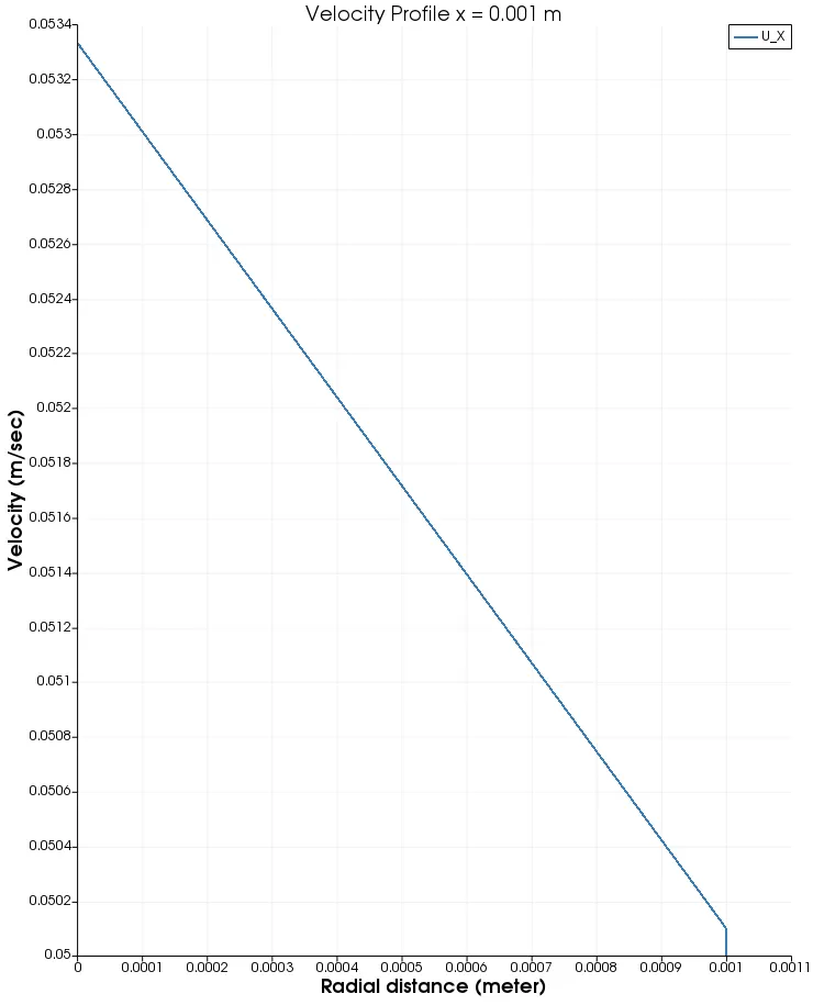
Here, we can see the inception of the boundary layer formation. The velocity is plotted from the axis to the wall of the pipe. So, the profile starts from the axis with velocity ≈0.791 m/s (maximum velocity) to 0 m/s at the wall. The velocity at the wall is 0 due to high shear stress. This is affected onto the flow to the adjacent fluid layers which are almost stationary due to the shear stress. As a result, the velocity gradient is non-uniform. Since this is near the hydrodynamic entry region, the boundary flow is slowly being initiated.
Velocity Profile x = 0.01 m/sec
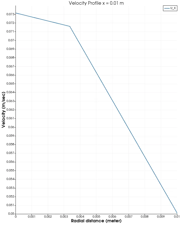
The above velocity profile at 0.01 meters belongs to the fully developed hydrodynamic flow region. Here, we can see the boundary layer forming and we have a unform velocity profile. We can easily observe that the profile is parabolic in nature. And the maximum velocity attained here is 0.0735 m/s. Similar to the 0.001 m snapshot, here we have negligible velocity at the wall due to the shear stress. We also observe that there is a lot of viscosity changes between the fluid layers.
Velocity Profile x = 0.02 m/sec
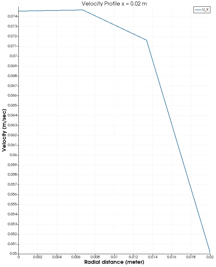
Now, we have the velocity profile at x = 0.02 meters. We observe similar trend when compared to the 0.01 m plot with the exception of more uniformity in the gradient. Here, the maximum velocity achieved is 0.0745 m/s. The location taken here is from the analytical value of the hydrodynamic entry length. We will see the fully developed flow near the exit of the pipe in the next snapshot.
Velocity Profile x = 0.05 m/sec
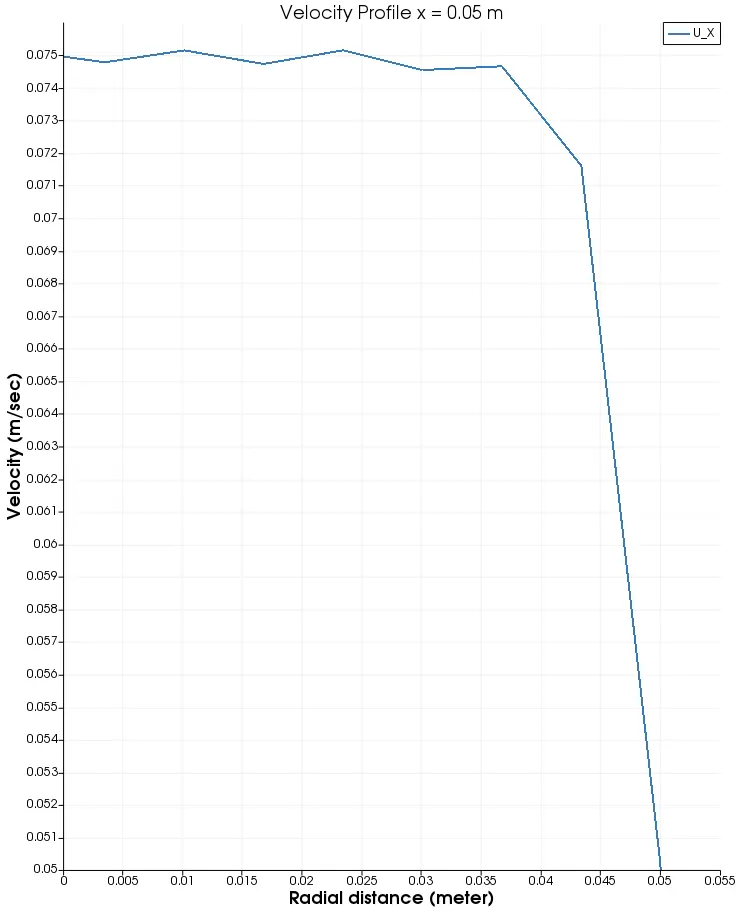
Above, we have a plot of the velocity profile at x-domain location of 0.05 meters. Here, the maximum velocity achieved is 0.075 m/s which is at the axis of the pipe. This plot was taken to observe and compare the velocity of fully developed flow near the exit of the pipe to the above plot of 0.02 m. The maximum velocity in 0.02 meters plot is 0.0745 m/s and in the above plot at 0.05 meters is 0.075 m/s which is very close.
Velocity Profile x = 0.1 m/sec
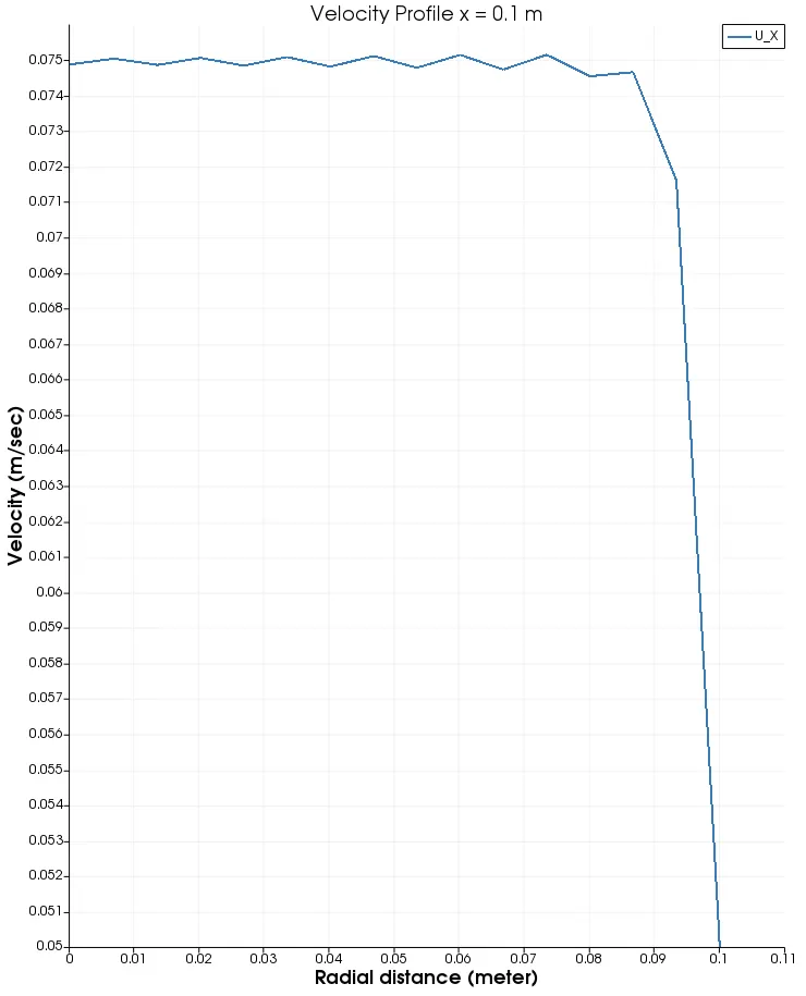
Above, we have a plot of the velocity profile at x-domain location of 0.1 meters. Here, the maximum velocity achieved is 0.0745 m/s which is at the axis of the pipe. This plot was taken to observe and compare the velocity of fully developed flow near the exit of the pipe to the above plot of 0.05 m. The maximum velocity in 0.05 meters plot is 0.075 m/s and in the above plot at 0.1 meters is 0.0745 m/s which is very close.
Pressure Profile :
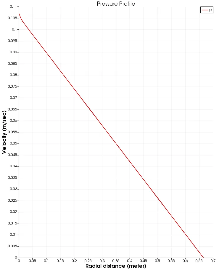
Now we observe the pressure profile captured along the pipe. And it is clearly evident that the pressure is decreasing as we move along the domain. This tells us that the pressure is high at the pipe entrance due to the non-uniformity in the velocity gradient due to high shear stress as we have observed in the above velocity profiles. The pressure naturally decreases as the velocity moves towards more uniformity where the boundary layers are uniform in nature. We can see the non-uniform pressure gradient till the hydrodynamic entry length. As the flow moves on, we see constant and uniform decrease in the pressure gradient compensating for the viscous forces in the flow. So, we can concur that the pressure drop is due to the viscous forces of the fluid. Here, the maximum pressure captured is about 1.108 pascals.
CONCLUSION:
We have automated the process of creating the blockMeshdict file for our simulations.
We have seen that the data obtained from the numerical simulation is very close to the analytical solutions.
REFERENCES: