Week 11 - Simulation of Flow through a pipe in OpenFoam
Aim :-
Simulate an axi-symmetric flow through a pipe in OpenFoam by applying the wedge boundary condition.
Objectives :-
1) Write code in Matlab to automate the generation of blockMeshDict file.
2) Validate Hydro-dynamic length with the numerical result.
3) Validate the fully developed flow velocity profile with its analytical profile.
4) Validate maximum velocity and pressured drop for fully developed flow.
5) Post-process Shear stress and validate wall shear stress for fully developed flow.
Theory :-
For the purpose of analysis, two reservoirs containing water (an incompressible Newtonian fluid) with surfaces at two different elevations were considered. A horizontal tube of length L with uniform round cross-section of radius R (diameter D = 2R) was used to connect the reservoirs such that water could flow among them. It was assumed that reservoirs were large enough such that changes in surface elevation would be very slow because of the flow into or out of the reservoirs. Therefore, the height of the fluid, and the associated hydrostatic pressure, in each reservoir was assumed to be constant for the purposes of analysis. It can safely be said that a constant pressure difference was maintained through-out between both reservoirs.
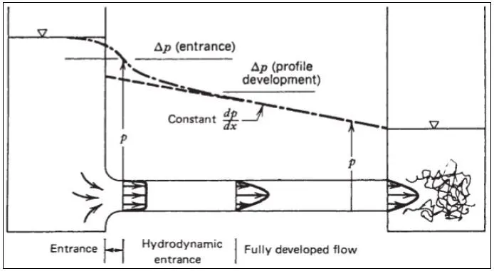
While flow advanced through the tube, effects of viscous shear stress gradually spread further away from the wall towards centre line. Continuity of flow warranted that mass flow rate at each cross-section of tube remained the same; therefore, the deceleration of the particles near the wall had to be catered by the acceleration of particles in the centre. Since the acceleration of the flow was dependent on the pressure forces, acceleration of centre particles warranted that the pressure kept on decreasing in the flow direction. Finally, once pressure forces and shear forces balanced out each other, the velocity profile became constant as the flow advanced through the pipe. In this condition, profile was fully developed with maximum velocity along the centre line and zero velocity along the wall.
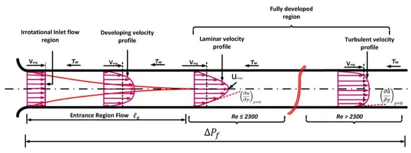
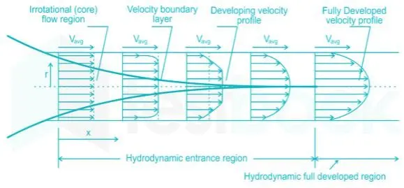
The region of the flow in which , the effects of the viscous shearing forces caused by fluid viscosity are felt , is called velocity boundary layer or just boundary layer. The hypothetical boundary layer divides the flow into 2 region : the boundary layer region (viscous effects and velocity changes are significant )and the irrotational flow region (frictional effects are insignificant and velocity remains constant in radial direction).
When the fluid just enters the pipe, the thickness of the boundary layer gradually increases from zero moving in the direction of fluid flow and eventually reaches the pipe center and fills the entire pipe. This region from the entrance of pipe to the point where the boundary layer covers the entire pipe is termed as the hydrodynamic entrance region and length of the pipe in this region is termed as the hydrodynamic entry length. In this region the velocity profile develops and thus the flow is called the hydrodynamically developing flow. After this region, the velocity profile is fully developed and continues unchanged. This region is called the hydrodynamically fully developed region.
Hagen Poiseuuiles Equation
In nonideal fluid dynamics, the Hagen–Poiseuille equation, also known as the Hagen–Poiseuille law, Poiseuille law or Poiseuille equation, is a physical law that gives the pressure drop in an incompressible and Newtonian fluid in laminar flow flowing through a long cylindrical pipe of constant cross section.
The assumptions of the equation are that the fluid is incompressible and Newtonian; the flow is laminar through a pipe of constant circular cross-section that is substantially longer than its diameter; and there is no acceleration of fluid in the pipe. For velocities and pipe diameters above a threshold, actual fluid flow is not laminar but turbulent, leading to larger pressure drops than calculated by the Hagen–Poiseuille equation.
Given below is the equation for hydrodynamic length for flow of Re<2300 .
`L_h /D ~= 0.05Re`
`L_h =`0.05*2100*0.005 = 0.525m
where D is the diameter of the pipe. (assumed value)
Total length of the pipe we consider = L>`L_h` = 0.1xRexD = 1.05m
Given below are equations for pressure drop for an incompressible laminar flow through a pipe .
`triangleP=P_1-P_2=(8muLV_(avg))/R^2 =(32muLV_(avg))/D^2`
Where,
`mu =`dynamic viscosity
L= length of the pipe
`V_(avg)`= average velocity
D= Diameter of the pipe.
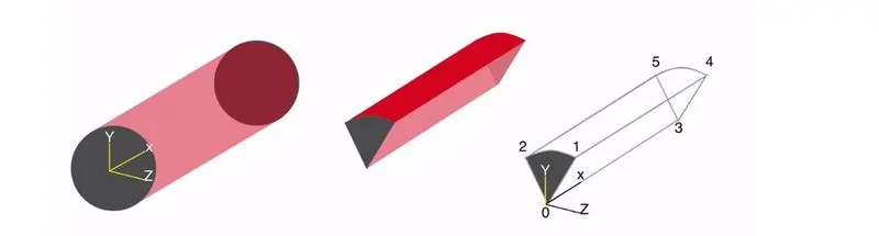
To make the calculation more easier, we have reduced the pipe into a wedge with an angle 3.
Codes and Explanations :-
MATLAB code to automate the generation of blockMeshDict file.
clear all
close all
clc

D=.005 ;
r=D/2 ;
L= 210*D ;
Re=2100 ;
theta=3 ;
a=sind(theta/2);
b=cosd(theta/2);
y=r*b;
z=r*a;

f1=fopen('blockMeshDict.txt','w');
fprintf(f1," /*--------------------------------*- C++ -*----------------------------------*\ \n");
fprintf(f1,"   =========                 | \n " );
fprintf(f1,"   \\      /  F ield         | OpenFOAM: The Open Source CFD Toolbox \n " );
fprintf(f1,"    \\    /   O peration     | Website:  https://openfoam.org \n " );
fprintf(f1,"     \\  /    A nd           | Version:  8 \n " );
fprintf(f1,"      \\/     M anipulation  | \n " );
fprintf(f1," \*---------------------------------------------------------------------------*/ \n " );
fprintf(f1," FoamFile \n " );
fprintf(f1," { \n " );
fprintf(f1,"     version     2.0; \n " );
fprintf(f1,"     format      ascii; \n " );
fprintf(f1,"     class       dictionary; \n " );
fprintf(f1,"     object      blockMeshDict; \n " );
fprintf(f1," } \n " );
fprintf(f1," // * * * * * * * * * * * * * * * * * * * * * * * * * * * * * * * * * * * * * // \n " );

fprintf(f1,"convertToMeters 1; \n");

fprintf(f1," vertices \n " );
fprintf(f1," ( \n " );
fprintf(f1,"     (0 0 0) \n " );               % Vertex 0
fprintf(f1,"     (0 %d %d) \n ",y,z );         % Vertex 1
fprintf(f1,"     (0 %d %d) \n ",y,-z );        % Vertex 2
fprintf(f1,"     (%d 0 0) \n ",L );            % Vertex 3
fprintf(f1,"     (%d %d %d) \n ",L,y,z );      % Vertex 4
fprintf(f1,"     (%d %d %d) \n ",L,y,-z );     % Vertex 5
fprintf(f1," ); \n " );

fprintf(f1," blocks \n " );
fprintf(f1," ( \n " );
fprintf(f1,"     hex (0 3 5 2 0 3 4 1) (200 50 1) simpleGrading (1 .1 1) \n " );
fprintf(f1," ); \n " );

fprintf(f1," edges \n " );
fprintf(f1," ( \n " );
fprintf(f1," ); \n " );

fprintf(f1," boundary \n " );
fprintf(f1," ( \n " );
fprintf(f1,"     inlet \n " );
fprintf(f1,"     { \n " );
fprintf(f1,"         type patch; \n " );
fprintf(f1,"         faces \n " );
fprintf(f1,"         ( \n " );
fprintf(f1,"             (0 1 2 0) \n " );
fprintf(f1,"         ); \n " );
fprintf(f1,"     } \n " );
fprintf(f1,"     outlet \n " );
fprintf(f1,"     { \n " );
fprintf(f1,"         type patch; \n " );
fprintf(f1,"         faces \n " );
fprintf(f1,"         ( \n " );
fprintf(f1,"             (3 5 4 3) \n " );
fprintf(f1,"         ); \n " );
fprintf(f1,"     } \n " );

fprintf(f1,"     topWall \n " );
fprintf(f1,"     { \n " );
fprintf(f1,"         type wall; \n " );
fprintf(f1,"         faces \n " );
fprintf(f1,"         ( \n " );
fprintf(f1,"             (1 4 5 2) \n " );
fprintf(f1,"         ); \n " );
fprintf(f1,"     } \n " );

fprintf(f1,"     axis \n " );
fprintf(f1,"     { \n " );
fprintf(f1,"         type empty; \n " );
fprintf(f1,"         faces \n " );
fprintf(f1,"         ( \n " );
fprintf(f1,"             (0 3 3 0) \n " );
fprintf(f1,"         ); \n " );
fprintf(f1,"     } \n " );

fprintf(f1,"     front \n " );
fprintf(f1,"     { \n " );
fprintf(f1,"         type wedge; \n " );
fprintf(f1,"         faces \n " );
fprintf(f1,"         ( \n " );
fprintf(f1,"             (0 3 4 1) \n " );
fprintf(f1,"         ); \n " );
fprintf(f1,"     } \n " );

fprintf(f1,"     back \n " );
fprintf(f1,"     { \n " );
fprintf(f1,"         type wedge; \n " );
fprintf(f1,"         faces \n " );
fprintf(f1,"         ( \n " );
fprintf(f1,"             (0 2 5 3) \n " );
fprintf(f1,"         ); \n " );
fprintf(f1,"     } \n " );


fprintf(f1," ); \n " );

fprintf(f1," mergePatchPairs \n " );
fprintf(f1," ( \n " );
fprintf(f1," ); \n " );
fprintf(f1,"  \n " );
fprintf(f1," // ************************************************************************* // \n " );
fclose(f1)
Output of MATLAB code, The blockMeshDict.txt file
 /*--------------------------------*- C++ -*----------------------------------*
   =========                 |
    \      /  F ield         | OpenFOAM: The Open Source CFD Toolbox
     \    /   O peration     | Website:  https://openfoam.org
      \  /    A nd           | Version:  8
       \/     M anipulation  |
  *---------------------------------------------------------------------------*/
  FoamFile
  {
      version     2.0;
      format      ascii;
      class       dictionary;
      object      blockMeshDict;
  }
  // * * * * * * * * * * * * * * * * * * * * * * * * * * * * * * * * * * * * * //
 convertToMeters 1;
 vertices
  (
      (0 0 0)
      (0 0.00249914 6.54424e-05)
      (0 0.00249914 -6.54424e-05)
      (1.05 0 0)
      (1.05 0.00249914 6.54424e-05)
      (1.05 0.00249914 -6.54424e-05)
  );
  blocks
  (
      hex (0 3 5 2 0 3 4 1) (200 50 1) simpleGrading (1 .1 1)
  );
  edges
  (
  );
  boundary
  (
      inlet
      {
          type patch;
          faces
          (
              (0 1 2 0)
          );
      }
      outlet
      {
          type patch;
          faces
          (
              (3 5 4 3)
          );
      }
      topWall
      {
          type wall;
          faces
          (
              (1 4 5 2)
          );
      }
      axis
      {
          type empty;
          faces
          (
              (0 3 3 0)
          );
      }
      front
      {
          type wedge;
          faces
          (
              (0 3 4 1)
          );
      }
      back
      {
          type wedge;
          faces
          (
              (0 2 5 3)
          );
      }
  );
  mergePatchPairs
  (
  );

  // ************************************************************************* //
The boundry conditons can be given as follows .
Velocity Boundary condition:-
/*--------------------------------*- C++ -*----------------------------------*\
  =========                 |
  \\      /  F ield         | OpenFOAM: The Open Source CFD Toolbox
   \\    /   O peration     | Website:  https://openfoam.org
    \\  /    A nd           | Version:  8
     \\/     M anipulation  |
\*---------------------------------------------------------------------------*/
FoamFile
{
    version     2.0;
    format      ascii;
    class       volVectorField;
    object      U;
}
// * * * * * * * * * * * * * * * * * * * * * * * * * * * * * * * * * * * * * //

dimensions      [0 1 -1 0 0 0 0];

internalField   uniform (0 0 0);

boundaryField
{
    inlet
    {
        type            fixedValue;
        value           uniform (0.42 0 0);
    }

    outlet
    {
        type            zeroGradient;
    }

    topWall
    {
        type            noSlip;
        value           uniform (0 0 0);
    }

    axis
    {
        type            empty;
    }

    front
    {
        type            wedge;
    }

    back
    {
        type            wedge;
    }
}

// ************************************************************************* //
Pressure Boundary Condition :-
/*--------------------------------*- C++ -*----------------------------------*\
  =========                 |
  \\      /  F ield         | OpenFOAM: The Open Source CFD Toolbox
   \\    /   O peration     | Website:  https://openfoam.org
    \\  /    A nd           | Version:  8
     \\/     M anipulation  |
\*---------------------------------------------------------------------------*/
FoamFile
{
    version     2.0;
    format      ascii;
    class       volScalarField;
    object      p;
}
// * * * * * * * * * * * * * * * * * * * * * * * * * * * * * * * * * * * * * //

dimensions      [0 2 -2 0 0 0 0];

internalField   uniform 0;

boundaryField
{
    inlet
    {
        type            zeroGradient;
    }

    outlet
    {
        type            fixedValue;
        value uniform 0 ;
    }

    topWall
    {
        type            zeroGradient;
    }

    axis
    {
        type            empty;
    }

    front
    {
        type            wedge;
    }

    back
    {
        type            wedge;
    }
}

// ************************************************************************* //
The data related to kinematic viscosity is updated in transportProperties file.
/*--------------------------------*- C++ -*----------------------------------*\
  =========                 |
  \\      /  F ield         | OpenFOAM: The Open Source CFD Toolbox
   \\    /   O peration     | Website:  https://openfoam.org
    \\  /    A nd           | Version:  8
     \\/     M anipulation  |
\*---------------------------------------------------------------------------*/
FoamFile
{
    version     2.0;
    format      ascii;
    class       dictionary;
    location    "constant";
    object      transportProperties;
}
// * * * * * * * * * * * * * * * * * * * * * * * * * * * * * * * * * * * * * //

nu              [0 2 -1 0 0 0 0] 1.0034e-6;


// ************************************************************************* //
The data related to simulation time duration and time step is updated in controlDict file as shown below:
/*--------------------------------*- C++ -*----------------------------------*\
  =========                 |
  \\      /  F ield         | OpenFOAM: The Open Source CFD Toolbox
   \\    /   O peration     | Website:  https://openfoam.org
    \\  /    A nd           | Version:  8
     \\/     M anipulation  |
\*---------------------------------------------------------------------------*/
FoamFile
{
    version     2.0;
    format      ascii;
    class       dictionary;
    location    "system";
    object      controlDict;
}
// * * * * * * * * * * * * * * * * * * * * * * * * * * * * * * * * * * * * * //

application     icoFoam;

startFrom       startTime;

startTime       0;

stopAt          endTime;

endTime         3;

deltaT          0.0001

writeControl    timeStep;

writeInterval   20;

purgeWrite      0;

writeFormat     ascii;

writePrecision  6;

writeCompression off;

timeFormat      general;

timePrecision   6;

runTimeModifiable true;


// ************************************************************************* //
OUTPUTS :-
Axi-symmetric flow was simulated and paraFoam view of the wedge was obtained .
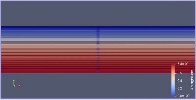
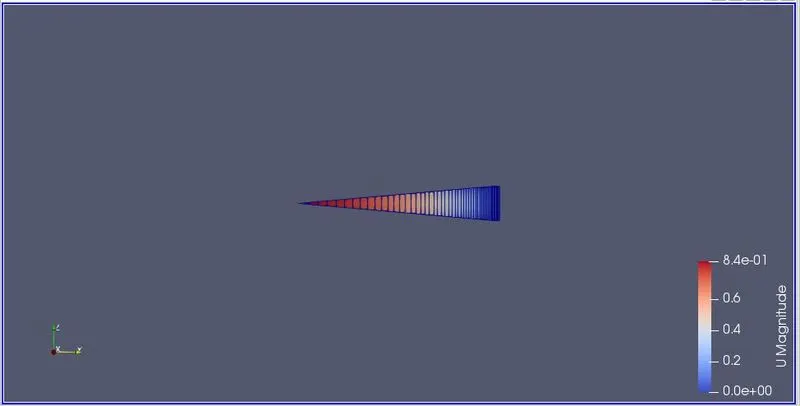
Velocity Profiles :-
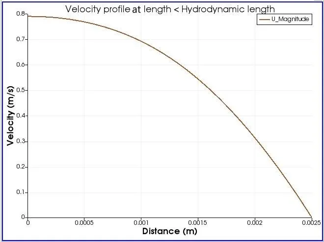
1) Velocity profile before forming fully developed flow
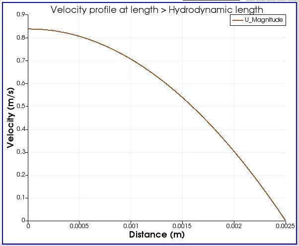
2) Velocity profile after attaining fully developed flow
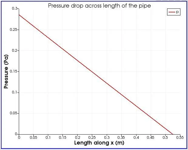
3) Pressure drop in the fully developed flow region.
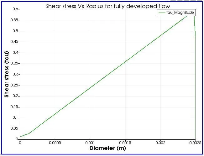
4) Wall shear stress for fully developed flow
RESULTS :-
1) When we look into velocity profile created at distance less than Hydrodynamic length, we can see that it is not fully develpoed because the maximum peak is at 0.79m/s . But when we see the velocity profile created at distance after the Hydrodynamic length, it is fully developed because the maximum peak is at 0.84m/s which is the maximum velocity and will not increase. We have only taken the half if we were taking the full profile the 1st will not give us a perfect parabolic shape were the 2nd will give a perfect parabola.
2) Fully developed flow velocity profile with its analytical profile.
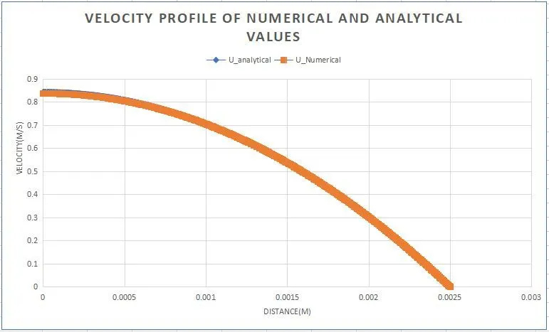
Looking into the graph we can see that the profile made with the Numerical value is matching the profile we made using Analytical value. That is why the numerical curve is almost overlapping the analytical curve.
3) Maximum velocity and pressured drop for fully developed flow
Maximum Velocity :-
Reynolds number = 2100
Working fluid used is water
Dynamic viscosity, `mu` = 1.0016e-3
Kinematic viscosity, `nu`= 1.0034e-6
Diameter, D =.005m
`V_(avg) = (Re*nu)/D =` (2100x1.0034e-6)/.005 = 0.42m/s
From velocity profile we can see that the Maximum velocity, Umax = 0.84m/s
Calculated Vavg = 0.42m/s
and , Umax = 2*Vavg = 2*0.42=0.84 m/s
So our graphical values matches the theroitical values.
Maximum Pressure Drop :-
From the graph the `triangleP` =0.28 Pa
`triangleP _(actual)= triangleP*rho`
Therefore,
`triangleP =` 0.28*1000 = 280 n/m^2
`triangleP_(analytical) = (32*mu*L*V_(avg))/D^2`
where,
L = Total length-Hydrodynamic length
=1.05-0.525 =0.525
Therefore,
`triangleP =` (32*1.0016*10^-3*0.525*0.42)/0.005^2 = 282.691584n/m^2
Hence we can say that graph is correct, because the value of pressure drop we got from the graph and the value we calculated are almost the same.
4) In our shear stress plot, the diameter 0m is the center of the pipe as we only take a part (wedge) of the real pipe . And the diameter 0.0025m is at the walls. As the walls are having no slip condition Maximum shear stress is at the walls and the shear stress at the center of the pipe is almost equal to zero.