week-11 Joint creation and Demonstration

Joint Creation and demonstration in LS-Dyna

1. Introduction

Joints are a vital part of any model, they are used to define the intended motion of parts with respect to each other. The correct modelling of joints is very important in FEA modelling to make an appropriate representation of the part or assembly with its functionality. In this project method of joint creation and their testing was done in LS-Dyna on simple geometries. The aim was to achieve proper constraints and motion in the components. Two models were used for each type of joint, one with rigid bodies and the other with deformable bodies. Various joints are discussed one by one in the following sections.

2. Cylindrical joint

A cylindrical joint is a two-degrees-of-freedom kinematic pair used in mechanisms. Cylindrical joints provide a single-axis sliding function as well as a single axis rotation, providing a way for two rigid bodies to translate and rotate freely.

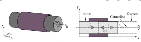
Fig 2.1: The representation of the cylindrical joint

In LS pre-post the shape modeller present in the mesh module was used to model two concentric cylinders made with shell elements as shown in the attached figure.

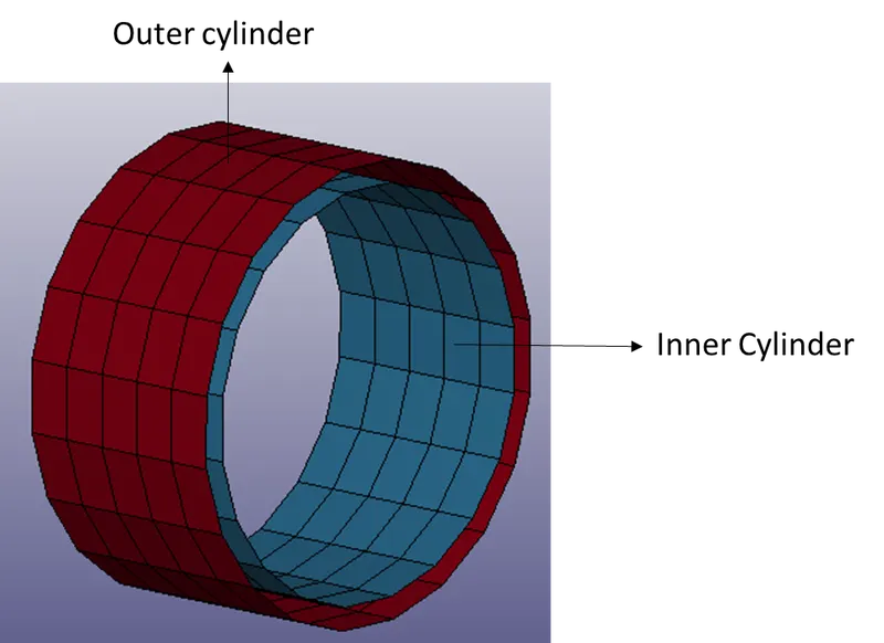
Fig 2.2: The geometry created in LS Pre-Post

For the first attempt we were going to model the parts as rigid bodies and for rigid bodies, we can place nodes outside of the body and make them belong to the body using *Constrained_Extra_Nodes. Four nodes were created at the centre of both ends as shown in the attached figure. Nodes 1,3 were assigned to the outer cylinder while pairs 2,4 were assigned to the inner cylinder using the constrained extra nodes keyword.

After that, a cylindrical joint was assigned to them using the constrained_joint_Cylindrical keyword. This keyword needs two pairs of coincident nodes out of which one needs to be from body 1 while the other from body 2.

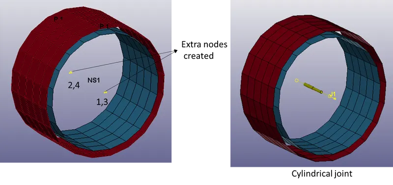
Fig 2.3: The cylindrical joint created in the LS Pre-post

Shell section card with 1 mm thickness was assigned to the cylinders. Then rigid material cards were assigned to the parts and CMO (Constrained motion option) was used for the outer body to make it fixed. For the inner cylinder, a rotation and translation boundary condition was used as shown in the attached figure.

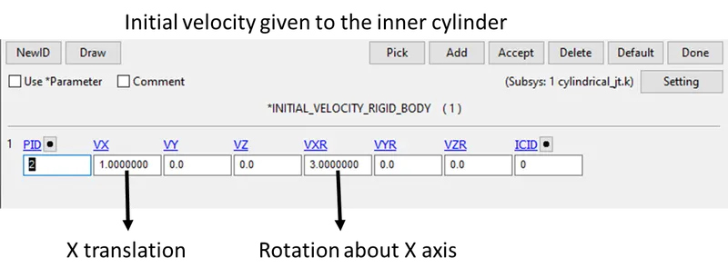
Fig 2.4: The boundary condition used for the inner cylinder

A termination time of 5 ms was used. The explicit solver tends to use a large timestep if no controls are used. This was prevented using *Control_Timestep card in the model as shown in the attached figure.

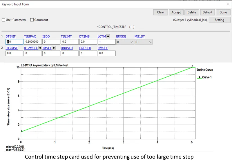
Fig 2.5: The control used for limiting the timestep size

2.1 MOdelling cylinders as deformable bodies

This time an elastic material was created as shown in the below figure and it was assigned to cylinders. For deformable bodies, the nodes outside of the body need to be modelled using constrained nodal rigid bodies.

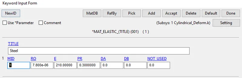
Fig 2.6: The material card used for the model

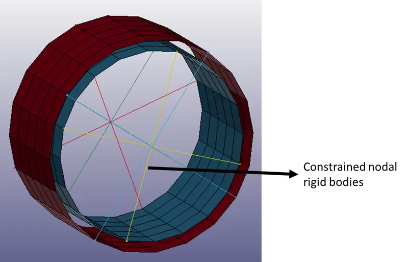
Fig 2.7: The constrained nodal rigid body used for connecting nodes outside the body

Then we need to constrain the outside cylinders using SPC (single point constraint) and provide initial velocity to the node-set containing all the nodes of the inner cylinder. The binary D3 plot was used to request output files.

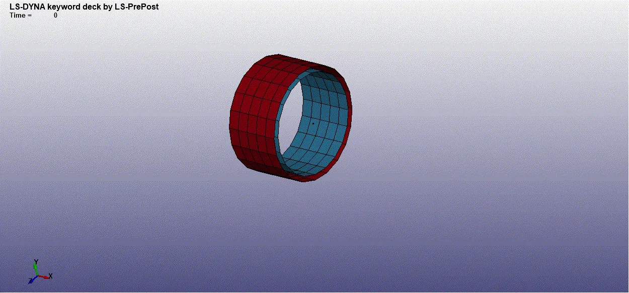
Animation 2.1.1: the cylindrical joint

As clear from the animation, rotation and translation of the inner cylinder was achieved.

3. Revolute Joint

A revolute joint (also called pin joint or hinge joint) is a one-degree-of-freedom kinematic pair used frequently in mechanisms and machines. The joint constrains the motion of two bodies to pure rotation along a common axis. The joint does not allow translation or sliding linear motion, a constraint not shown in the diagram. Almost all assemblies of multiple moving bodies include revolute joints in their designs. Revolute joints are used in numerous applications such as door hinges, mechanisms, and other uni-axial rotation devices.

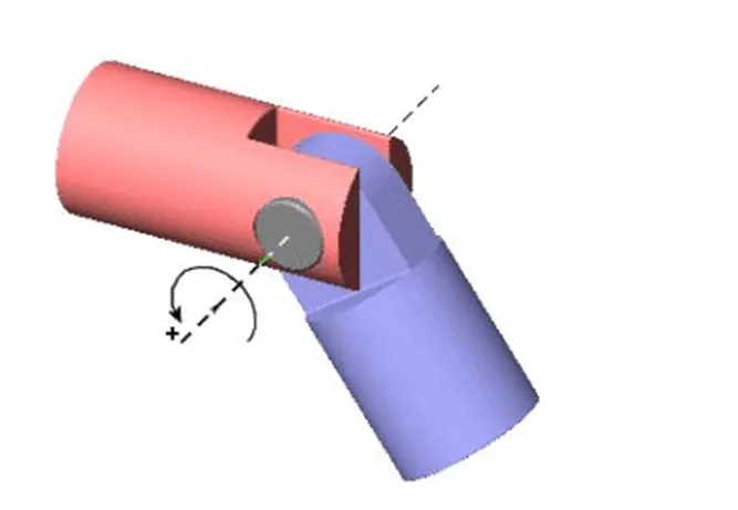
Fig 3.1: The revolute joint

Two rectangular plates were modelled with shape mesher and they were assigned shell section with 1 mm thickness. Then two rigid material cards were created and in one that was assigned to the left side, CMO was used to constrain it.

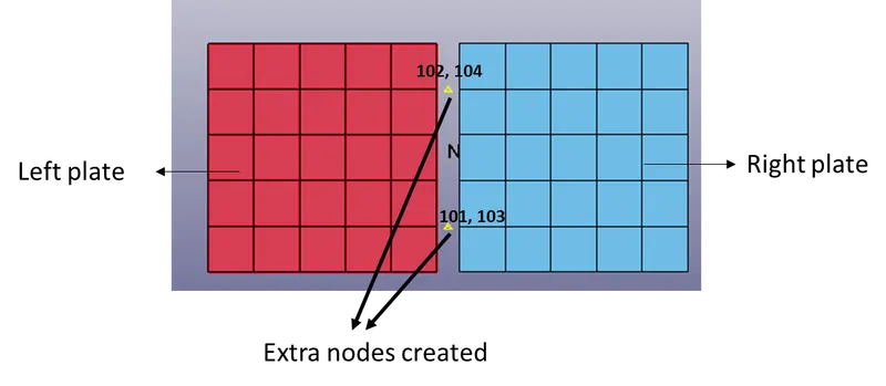
Fig 3.2: The Geometry for revolute joint

Then the revolute joint was modelled using the node sets in a manner similar to the cylindrical joint. A velocity in the Z direction(normal to screen) was assigned to nodes of the right plate as shown in the attached figure.

Fig 3.3: The revolute joint and the velocity card used

Again the control timestep and control termination cards were used similar to the cylindrical joint.

3.1 Modelling as deformable bodies

An elastic material card as shown in fig 2.6 was used for both plates. This time again the outside nodes need to be modelled along with constrained nodal rigid bodies as shown in the attached figure. Then we need to constrain the left plate using SPC as done in the case of a cylindrical joint with a deformable body.

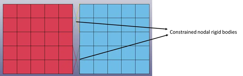
Fig 3.1.1: The constrained nodal rigid bodies used for connecting nodes outside the body

Animation 3.1.1: The animation joint

4. Spherical joint

The spherical joint, also known as a ball-and-socket joint, allows three relative rotations between the two connected segments and is frequently used to model the hip and glenohumeral joints. It gives three degrees of freedom which are all the rotations.

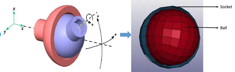
Fig 4.1: The FE model of ball and socket

In the shape mesher ball and socket were modelled with shell mesh as shown in the above figure. For a spherical joint, a set of two nodes that belong to the ball and socket respectively need to be constrained. So two nodes were created at the centre and *Constrained_extra_node card was used to assign them to ball and socket respectively.

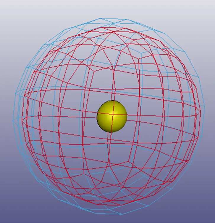
Fig 4.2: The spherical joint

Then two rigid material cards were created and one was used for each. The rigid card used for the socket was constrained using the CMO option and ball was provided with rotation in a manner similar to previous joints.

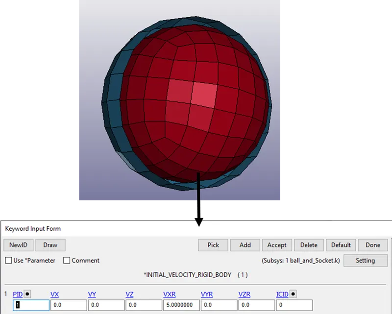
Fig 4.3: The BC used for the model

4.1 Modelling with deformable body

Again elastic material was assigned to the parts and CNRB was created to join the nodes at the centre to ball and socket respectively. Rest all the things were similar to the above cases.

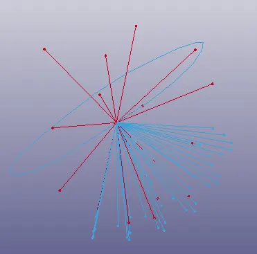
Fig 4.1.1: The CNRB used for connecting nodes to the body.

Animation 4.1.1: The spherical joint

5. Translational joint

A translational joint allows translational movement of two bodies in the direction of a vector defined between the bodies. A translational joint constrains rotational motion in all directions and only allows translational motion in the direction of a specified vector. This means it has only one degree of freedom and constrains the other five degrees of freedom. You can also constrain the motion of two bodies by expressing the translational degree of freedom as a function of time.

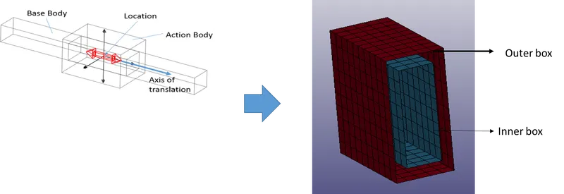
Fig 5.1: the translational joint

The modelling of translational joint requires three-node pairs out of which two needs to be collinear and the third one needs to deviate from the line joining the other two. Setup is shown in the below-attached figure.

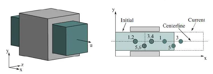
Fig 5.2: the translational joint details

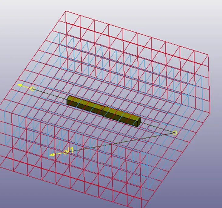
Fig 5.3: The translational joint with rigid bodies

5.1 Modelling with deformable body

Again CNRB were used for modelling the connection between the out of the body nodes.

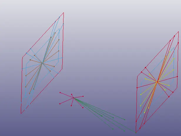
Fig 5.1.1: The CNRB used for modelling nodes outside the body

Animation 5.1.1: the motion of translational joint

As clear from the animation the rotations are not allowed and translation is happening so we were successful in this joint modelling.