week-11 Joint creation and Demonstration
Joint Creation and Demonstration in LS DYNA:
A joint is a section or sub-assembly used to connect two parts (linkages) with a relative motion between the connected parts. The joint can either be a fully constrained and partial constrained i.e free movement. The demonstration presented here comprises of creation and working of joints between simple parts (both rigid and flexible in nature) and these can be extended to complex parts although the principle remains same.
Defining joints using extra node/node set (For rigid bodies):
Joints in LS DYNA can be defined using extra nodeset methods, provided the bodies are rigid in nature.
In this method, nodes which are co-incident are created. These nodes are associated with the rigid bodies using Constrained_Extra_node_set keyword.
Then joint is defined using the extra nodes associated with the parts using Contrained_joint_.
1. Translational joint: The relative motion between bodies has only degree of freedom i.e along the axial direction. Three sets of nodes are required to define this joint. Two sets for allowing the motion, one set for constraining the rotational degree of freedom.
Accordingly, three sets of co-incident nodes are created at three points and respective sets are associated with parts.
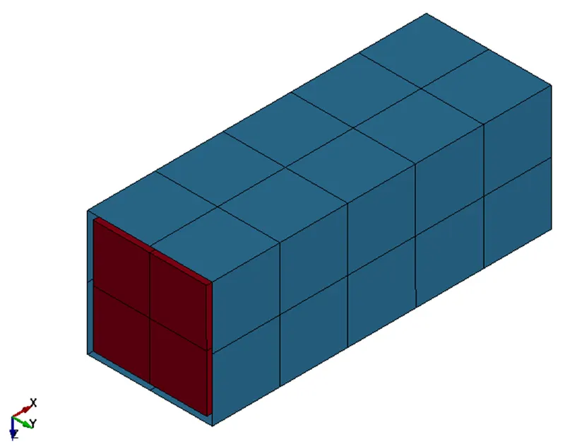
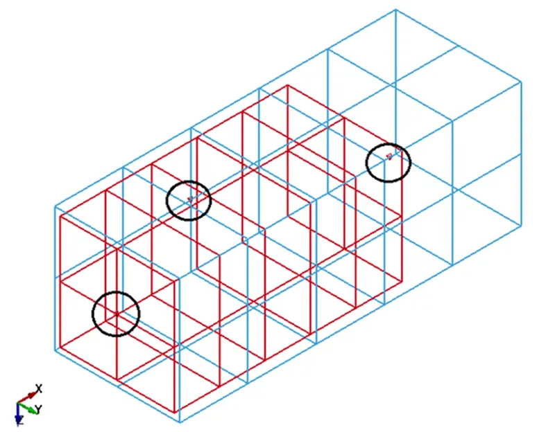
Three pair of nodes numbered 1001,1002,1003 are associated with the solid tube and nodes 2001,2002,2003 are associated with shell tube.
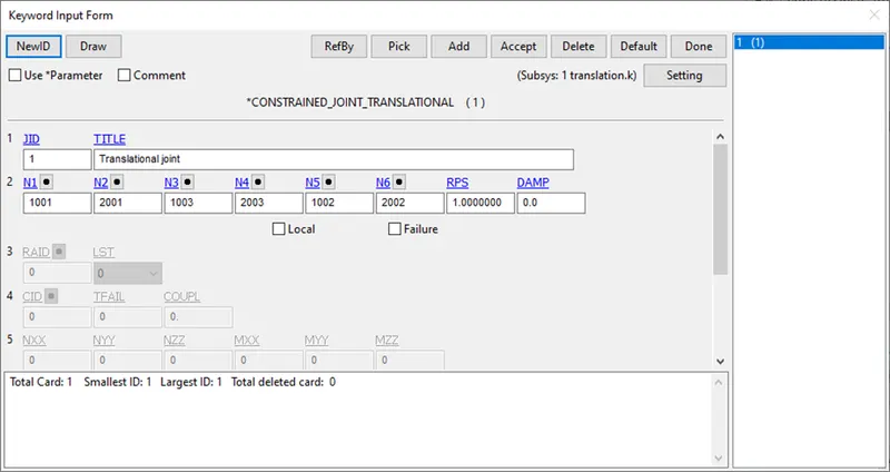
Joint is defined using Joint_Translation
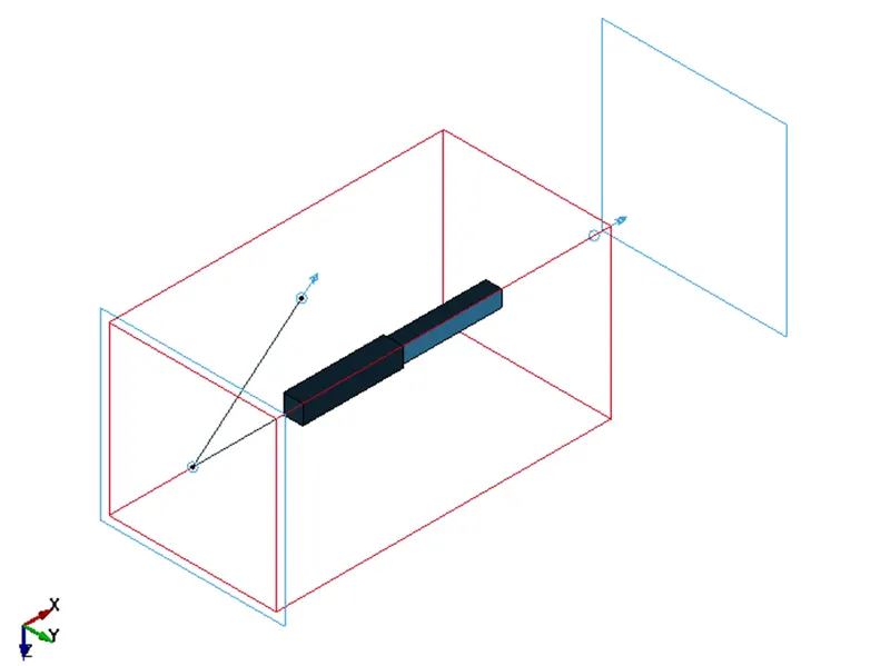
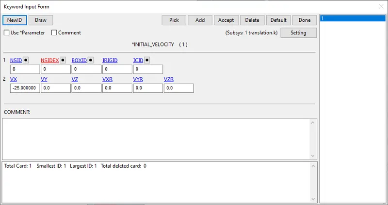
Boundary condition used: Since a rigid card was used the shell was fixed/constrained using the MAT_20 rigid material keyword. The solid tube was given using Initial_velocity_generation keyword for the part in negative x direction.
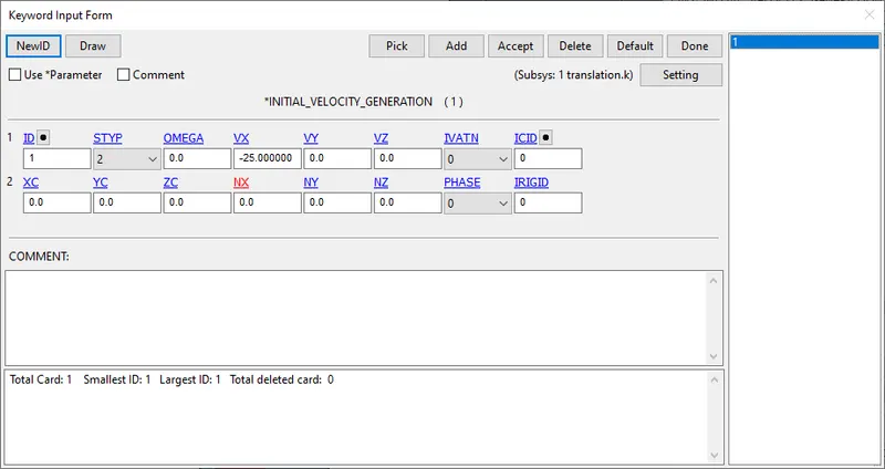
2. Cylindrical joint: The relative motion between bodies has two degrees of freedom, i.e one axial and 1 rotational dof. Only two sets of nodes are required to define the cylindrical joint for rotational degree of freedom and axial movement can be provided using the Velocity_rigid_motion.
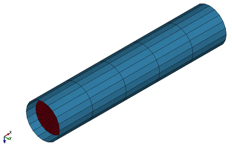
Two sets of nodes are defined at two points and respective sets are associated with parts.
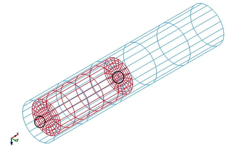
Nodes numbered 1001, 1002 are associated with solid tube and nodes 2001,2002 are associated with shell tube.
Joint is defined using Joint_Cylindrical
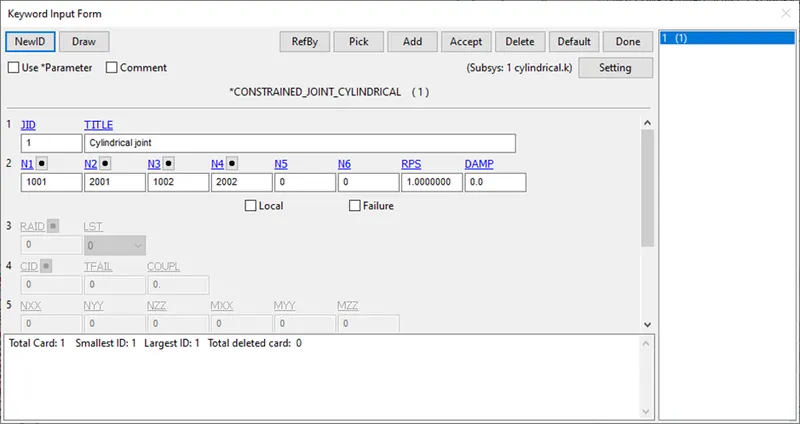
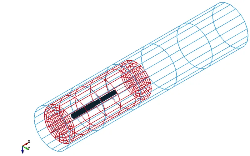
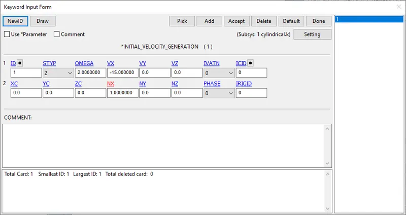
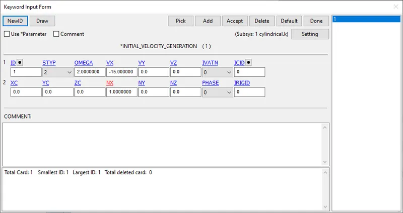
Boundary condition used: Since a rigid card was used the shell was fixed/constrained using the MAT_20 rigid material keyword. The solid tube was given using Initial_velocity_generation keyword for the part in negative x direction (axial) and rotational velocity (omega) about the x direction.
3. Revolute joint: This joint is also known as hinge joint or pin joint. In this case the relative motion between bodies is restricted to rotations about the axis formed by pair of co-incident nodes.
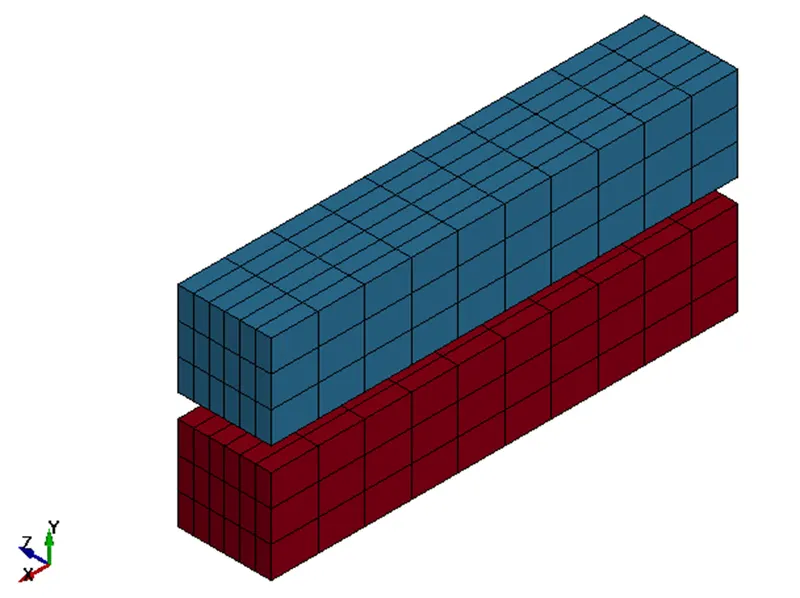
One sets of nodes are defined and respective sets are associated with parts for each of the revolute joint.
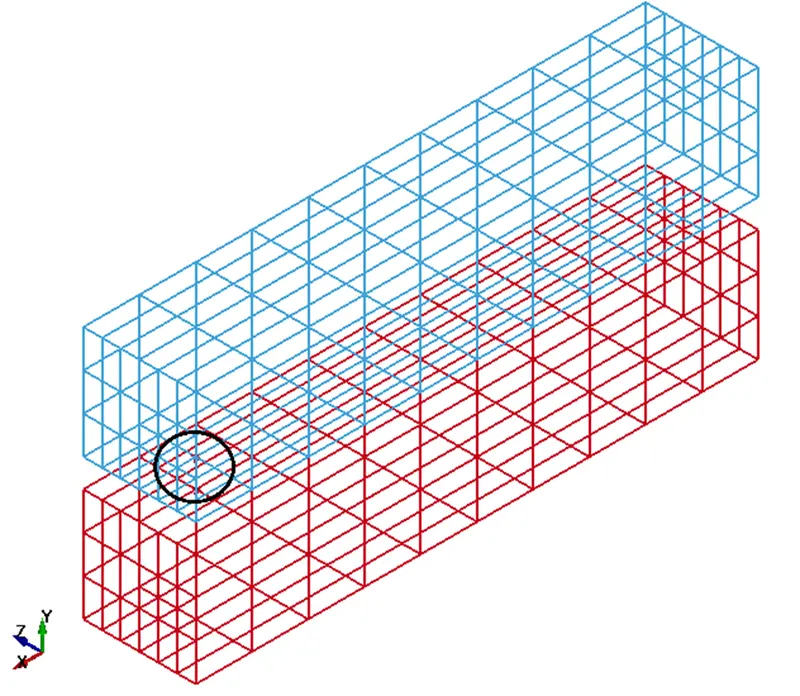
Joint is defined using Joint_Revolute
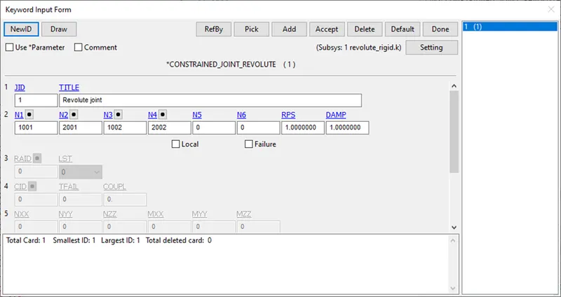
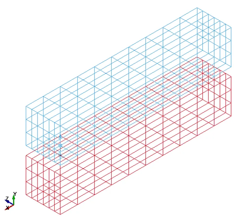
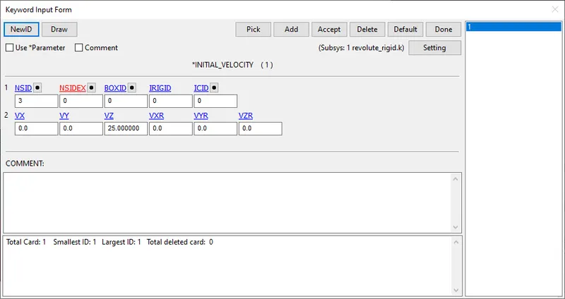
Boundary condition used: Since a rigid card was used the bar(red colour) was fixed/constrained using the MAT_20 rigid material keyword. A Initial_velocity card was defined after creating a nodeset consisting of edge nodes to impart the velocity to the moving bar.
4. Spherical joint: In this joint, the relative motion between two bodies is free in all rotational degree of freedom but constrained in translational degree of freedom. Defining this joint in LS DYNA requires one set of nodes.
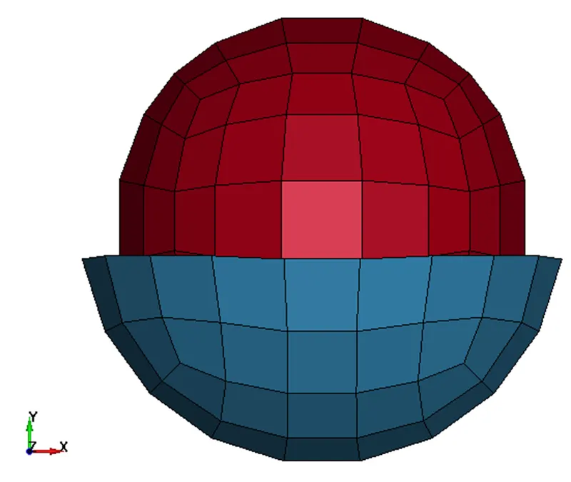
A pair of co-incident nodes are created at the centre of the solid sphere.
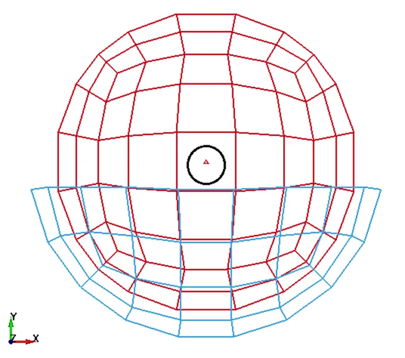
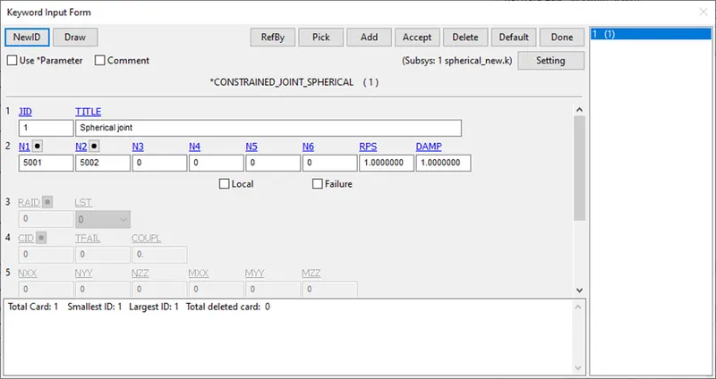
Extra_nodes_node is defined to associate the nodes created at the centre of the solid sphere. Node 5001 is associated with solid sphere and 5002 are associated with the shell.
Joint is defined using Joint_Spherical.
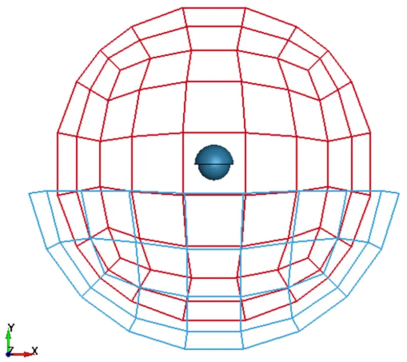
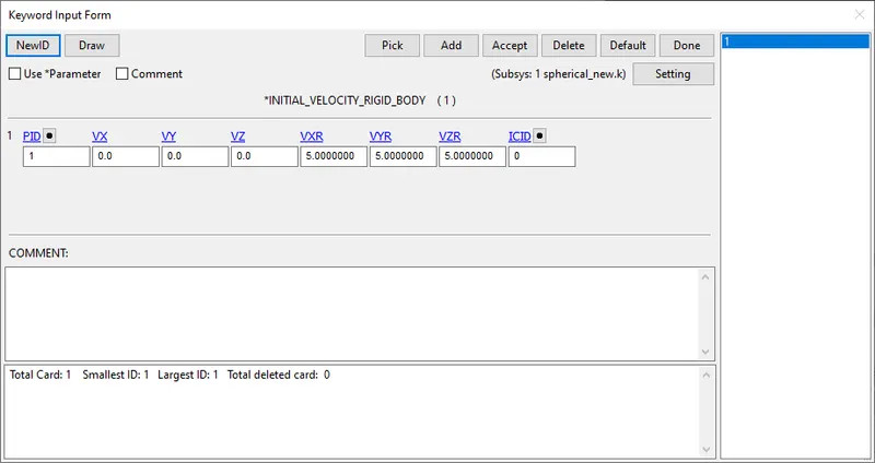
Boundary condition used: Since a rigid card was used, the shell was fixed/constrained using the MAT_20 rigid material keyword. The solid sphere was given rotational velocity about x, y, z direction.
Defining joints using Constrained nodal rigid body(CNRB) (For flexible bodies):
Another way to define joints is by using Constrained nodal rigid body(CNRB). This is used to define joints among the deformable bodies. Just like the constrained extra node set, cnrb are defined to associate the nodeset with the parts. Then joints are then defined using Contrained_joint_.
Constrained nodal rigid body are created from Entity creation tab, selecting all the nodes of the part and the additional node created for defining the joint.
1. Translational joint:
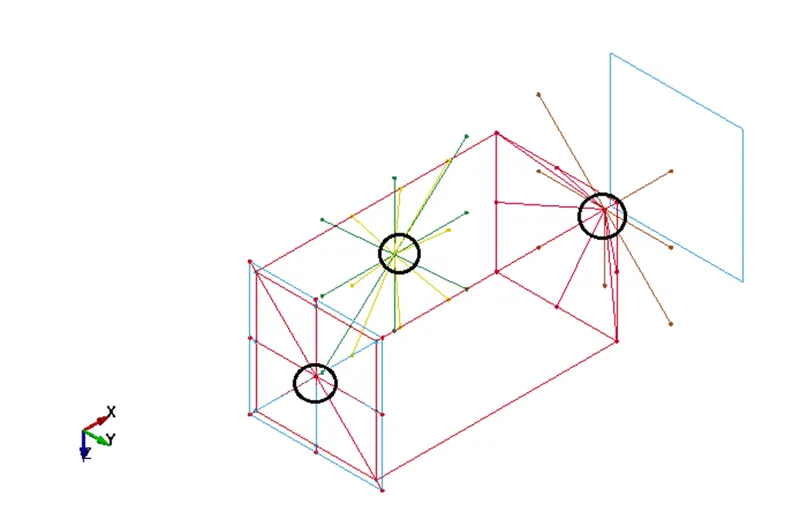
The CNRB are created with nodes selected in the neighbouring elements and a node used to define the joint. The rest of the boundary conditions are applied with due considerations to the deformable bodies.
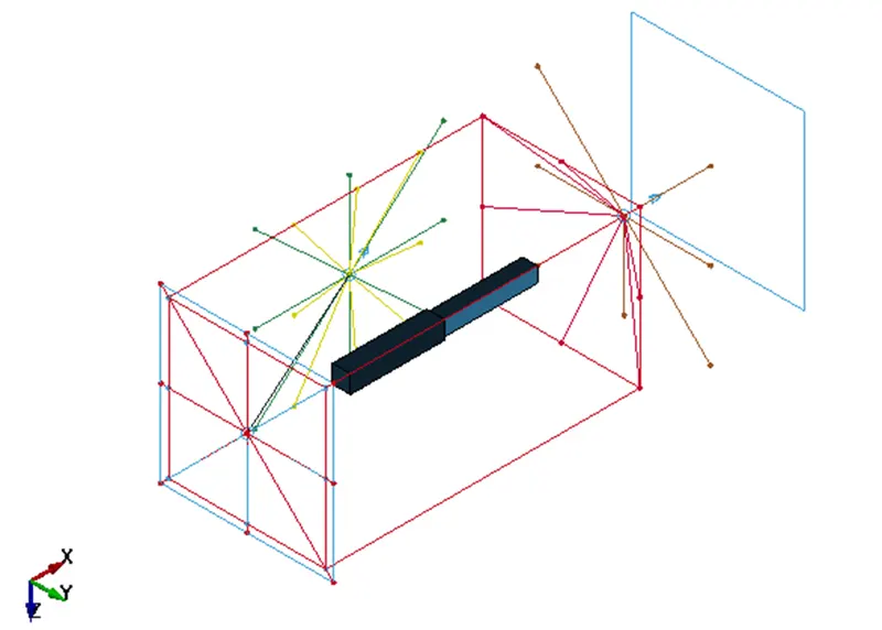
Boundary conditions: A Spc_set card was used to fix the hollow shell nodes, and Initial_velocity card was used to impart the velocity to solid tube using nodeset.
2. Cylindrical joint:
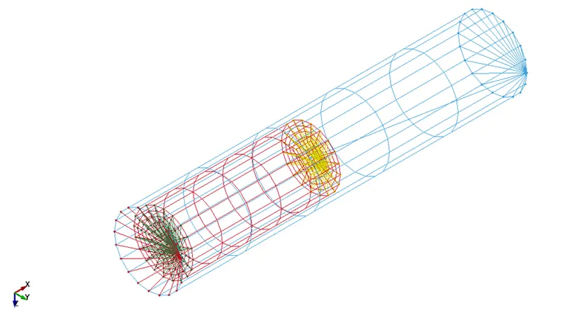
Joint is created using Constrained_joint_cylindrical to assign the corresponding node numbers.
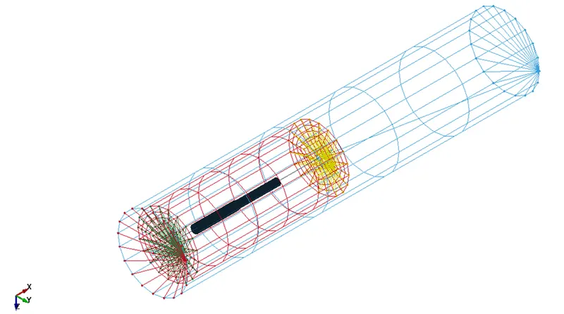
Boundary conditions: A Spc_set card was used to fix the hollow shell nodes, and velocity_generation card was used to impart the velocity (axial and rotational) to solid tube using nodeset.
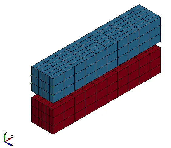
3.Revolute joint:
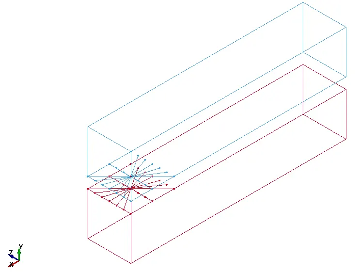
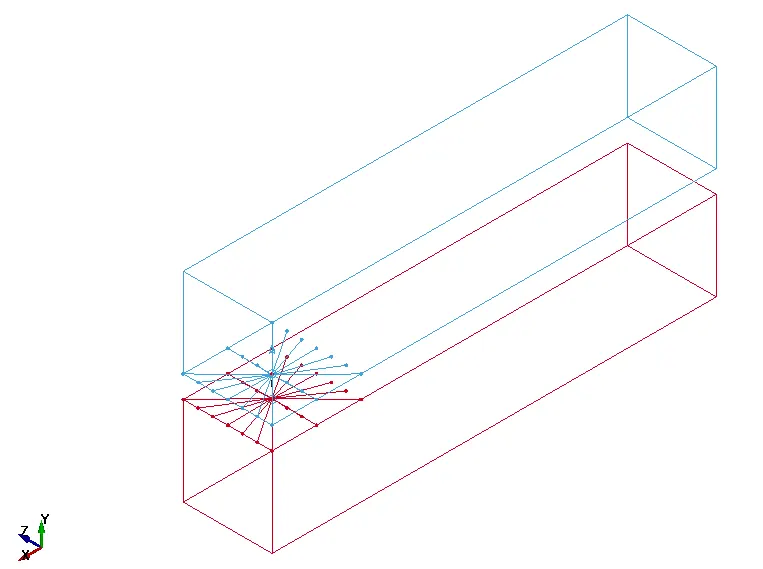
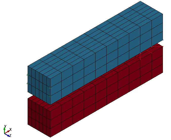
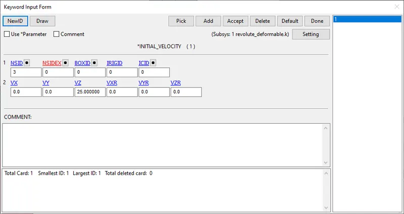
Boundary conditions: A Spc_set card was used to fix the solid nodes (part 1, red colour), initial_velocity card is used to impart the velocity to the edge nodes using nodeset.
4.Spherical joint:
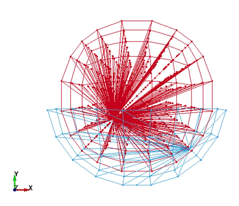
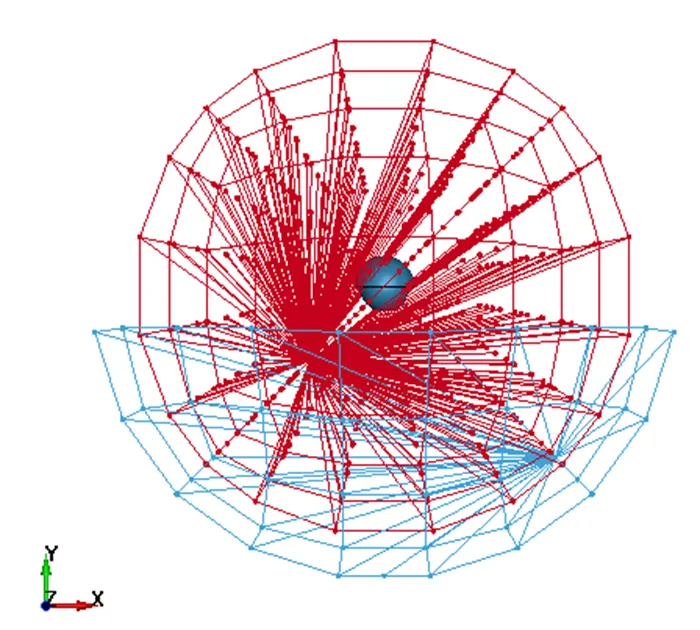
Boundary conditions: A Spc_set card was used to fix the shell nodes, three initial_velocity_generation cards are used to impart the rotational velocity in each of the directions(x,y,z) for the solid sphere as a part.
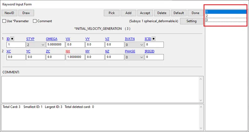
Boundary conditions:
For defining joints in case of rigid bodies, partial boundary conditions are imparted using Mat_Rigid material card.
In case of deformable bodies, Spc_set are defined to fix the bodies.
Velocity conditions are used to define relative motion of the moving parts. Prescribed_motion_set and Initial_velocity_Rigid and Initial_velocity_generation keywords are used for the purpose. Care has been taken to specify the same values/parameters while defining the boundary conditions.
Control_termination keyword is used to denote the endtime of the simulation.
Database:
Binary_d3plot is defined to output the result at 0.1 intervals of endtime.
Animation plots of the different joints:
1. Translational joint:
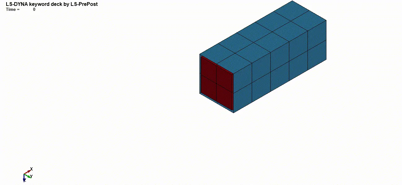
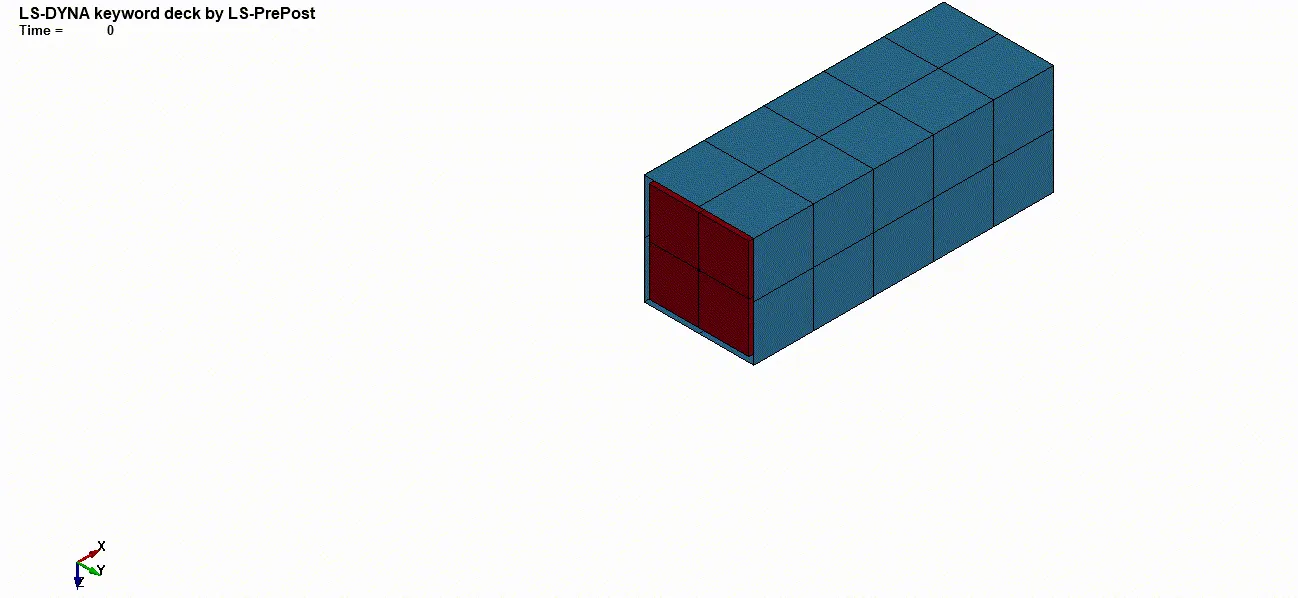
Rigid bodies Flexible bodies
2. Cylindrical joint:
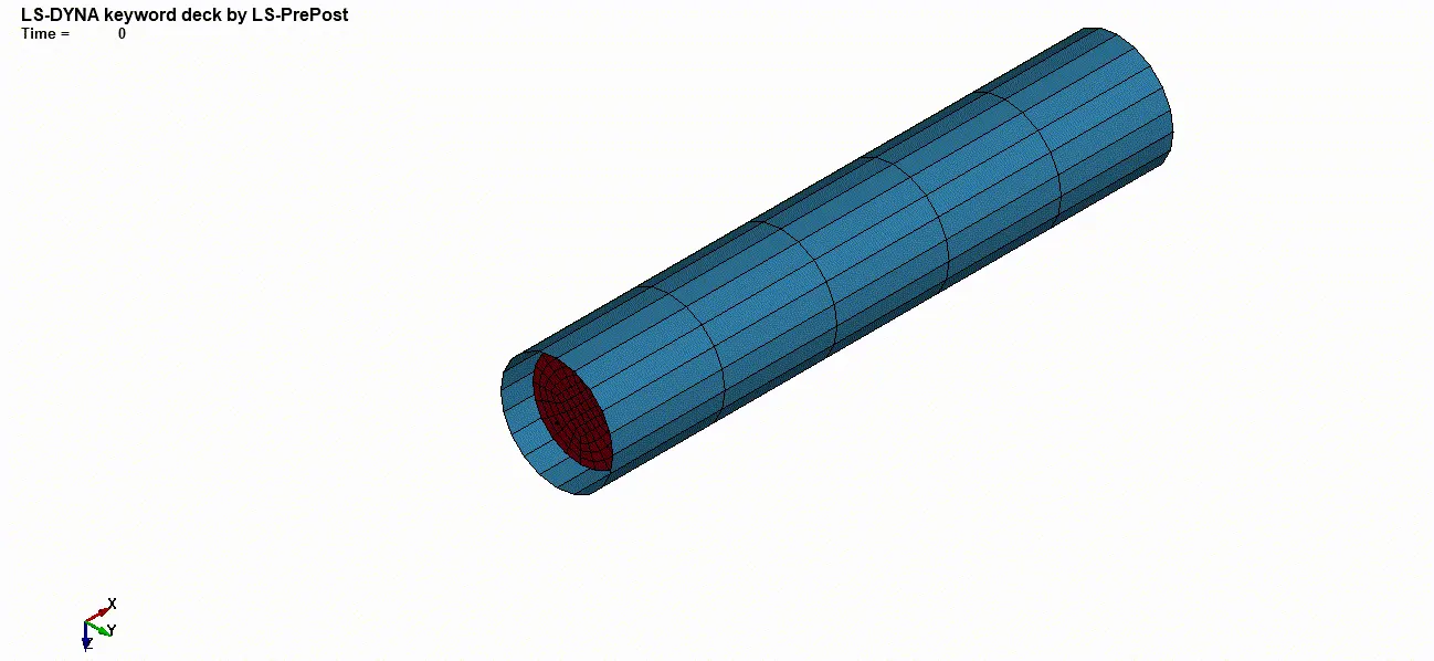
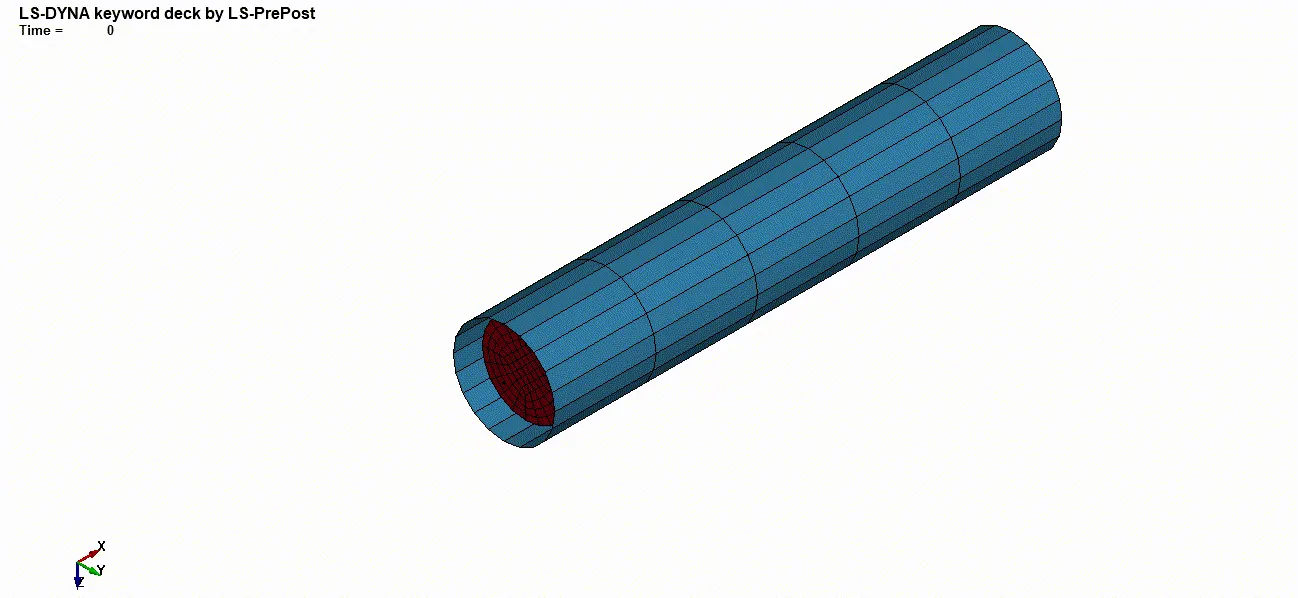
Rigid bodies Flexible bodies
3. Revolute joint:
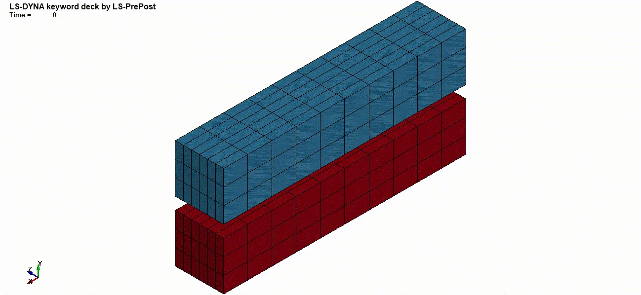
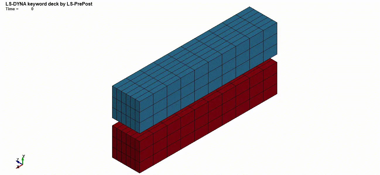
Rigid bodies Flexible bodies
4. Spherical joint:
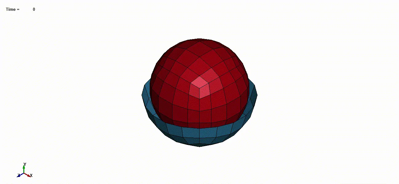
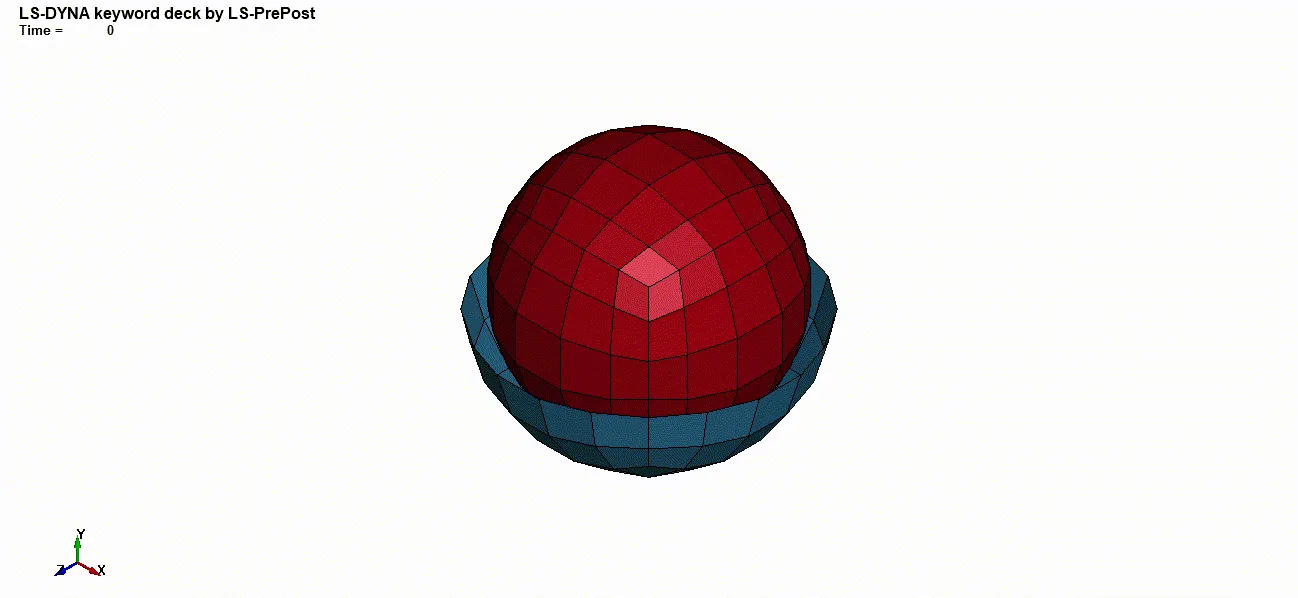
Rigid bodies Flexible bodies
Conclusion:
Defining and creation of joints were demonstrated for both rigid and flexible bodies. The major difference between them is the association of extra nodes to the respective parts in case of of rigid bodies and creation of CNRB with the extra nodes in case of flexible bodeis. The boundary conditions have to be changed accordingly in both cases as per the case.
Please follow the link to access the input, output and animation files : https://drive.google.com/drive/folders/1Bki2pQk8TAeCHyDusmFt6Q3VocpKE3Rx?usp=sharing