Week 11 Challenge: Joint Creation and demonstration Challenge

Course: LS-DYNA for Structural Mechanics/ FEA

Submitted by: Amanpreet Singh Whan

Supervisor: Tholkappiyan D

October 13, 2021

Table of Contents

1 Introduction.

2 Aims.

3 Methodology.

4 Results.

5 Conclusion.

1 Introduction

LS-DYNA is an advanced general-purpose multiphysics simulation software package developed by the former Livermore Software Technology Corporation (LSTC), which was acquired by Ansys in 2019. While the package continues to contain more and more possibilities for the calculation of many complex real-world problems, its origins and core competency lie in highly nonlinear transient dynamic finite element analysis (FEA) using explicit time integration. LS-DYNA is used by the automobile, aerospace, construction and civil engineering, military, manufacturing, and bioengineering industries.

The purpose of the Week 11 challenge is to demonstrate spherical, revolute, cylindrical, and translational joints between two rigid bodies and two deformable bodies. Several joints are available in LS-DYNA that can be defined between two rigid bodies or nodal rigid bodies. The difficult part of the joint definition from the pre-processing point of view is the creating of nodes that define the joint axes and subsequent merging of them to the respective rigid bodies. The available different constrained joints in LS DYNA are discussed below.

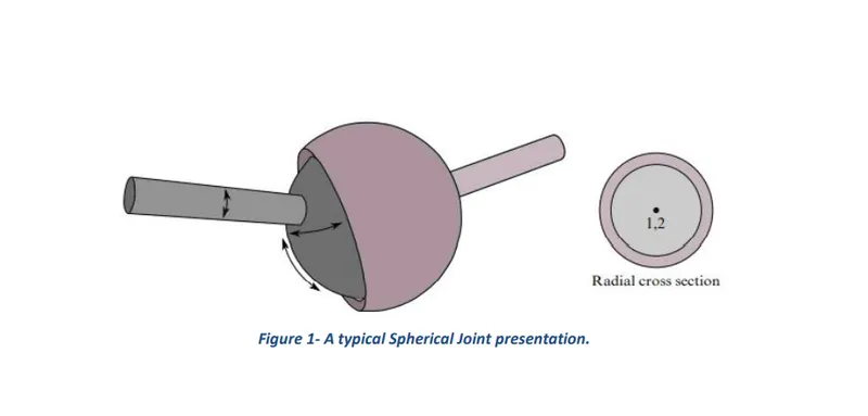
Spherical Joint: The relative motion of the rigid bodies is constrained so that nodes that are initially coincident remain coincident. In the below figure, the socket’s node is not interior to the socket—LS-DYNA does not require that a rigid body’s nodes be interior to the body.

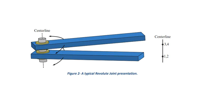
Revolute Joint: Nodes 1 and 2 are coincident; nodes 3 and 4 are coincident. Nodes 1 and 3 belong to rigid body A; nodes 2 and 4 belong to rigid body B. The relative motion of the two rigid bodies is restricted to rotations about the axis formed by the two pairs of coincident nodes. This axis is labeled the “centerline.”

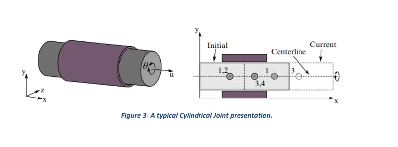
Cylindrical joint: This joint is derived from the rotational joint by relaxing the constraints along the centerline. This joint admits relative rotation and translation along the centerline.

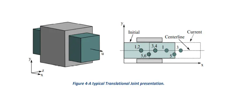
Translational Joint: This is a cylindrical joint with the third pair of off-centerline nodes which restrict rotation. Aside from translation along the centerline, the two rigid bodies are stuck together.

2 Aims

Demonstrate spherical, revolute, cylindrical, and translational joints between two rigid bodies and two deformable bodies.

3 Methodology

The section describes different stages that were performed to set up the simulation file using an engineering tool LS-DYNA for the completion of the Week 11 Challenge task. These stages can be broadly categorized into creating an input deck containing different cards such as contact, control, database, element, hourglass, Boundary condition, keyword, MAT, node, part, section, and title.

Since LS-DYNA does not have a default system of units, therefore, the user needs to input material properties and physical dimensions according to a consistent system of units as per their choice. Considering the challenge requirements of demonstrating various joints between two rigid and deformable parts, kg mm ms were assumed to be the most appropriate units.

In general, the following procedure has to be followed to deploy any constraint joint between two bodies irrespective of their nature in LS DYNA. What follows hereafter is the process that was carried out to create a revolute joint between two rigid and two deformable bodies. Subsequently, the same steps were repeated for creating cylindrical, spherical, and translational joints between two rigid bodies and two deformable bodies.

Procedure for creating a revolute Joint between 2 Rigid and Deformable parts

Step 1)- Creating Geometry for Revolute Joint

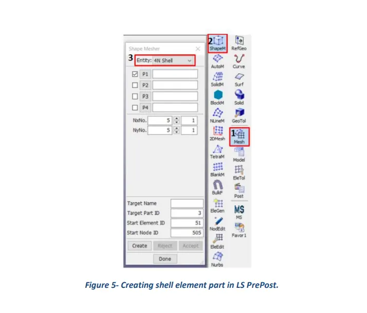
• Two separate shell elements were created using the Element and Shape>Mesher option available in LS-PrePost. Select the entity as 4N shell and assign the node coordinates for a shell element with the required mesh density. The following figure shows the option available in LS Dyna.

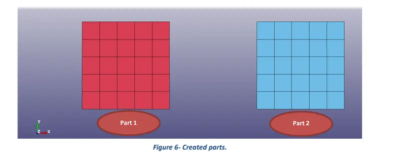
• Some free space was kept between two parts for a better presentation of a revolute joint. The following figure depicts the created parts in the LS PrePost for the revolute joint.

Step2)- Creating revolute joint between 2 Rigid Bodies

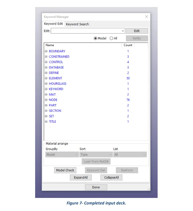
• Create material, sections, and other relevant cards and assign appropriate values to their parameters for simulation purposes.

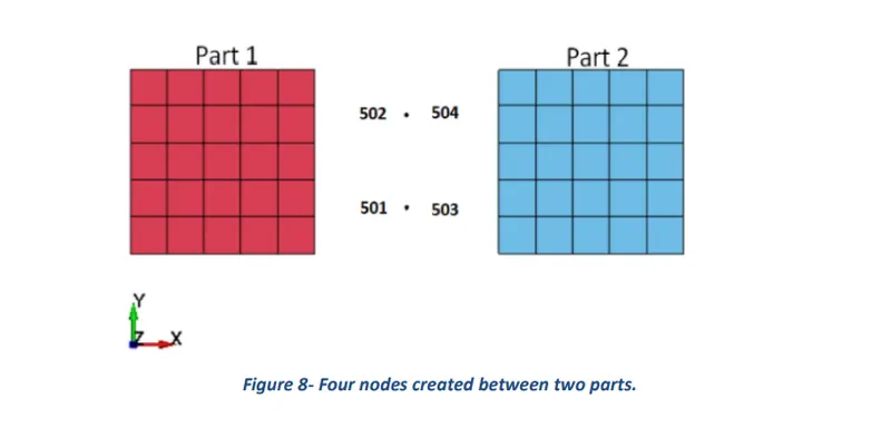
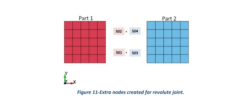
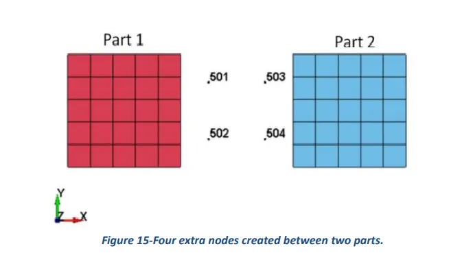
• Create four extra nodes manually which are further needed to be associated with two parts for making a revolute joint. Create nodes by Element Tools>Node editing option and give distinct node IDs for all four nodes. Number the nodes as 501, 502, 503, and 504.
• Nodes 501 and 503 are coincident and 502 and 504 are coincident. The same analogy has been used as shown in figure 2. The following figure 8 shows the location of four newly generated ones.

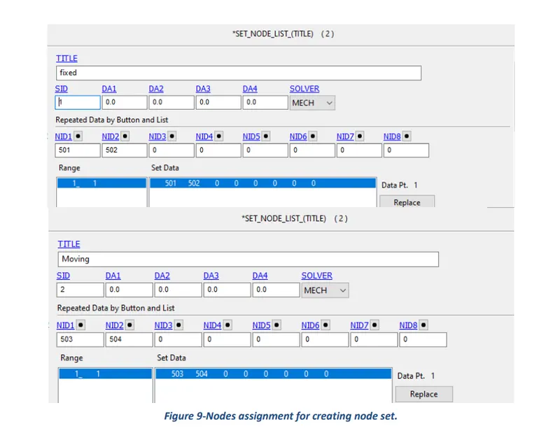
• Create new node sets, where nodes 501 and 502 belong to one node-set, and 503 and 504 nodes belong to another node-set. Figure 9 shows the node assignment for the Set_Node_List keyword. The node sets can be created through Create Entity>Set Data>Set Node>Create option.

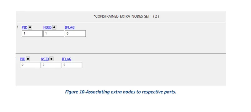
• These newly created nodes are in the space and do not belong to any of the parts now. So, for associating these nodes with part 1 and part 2, Constarined_Extra_Nodes_set is used. Figure 10 shows that nodes 501 and 502 belong to part 1, and nodes 503 and 504 belong to part 2.

• The figure depicts the four nodes, and the respective nodes are highlighted with the same part color to which they are associated.

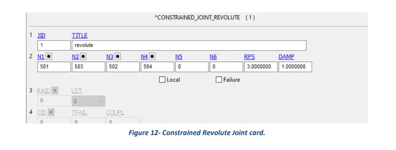
• The revolute joint was defined by using the Constrainted_Joint_Revolute keyword. Four nodes should be defined to create a revolute joint. N1 (501) and N3 (503) belong to part 1, and N2 (502) and N4 (504) belong to part 4.

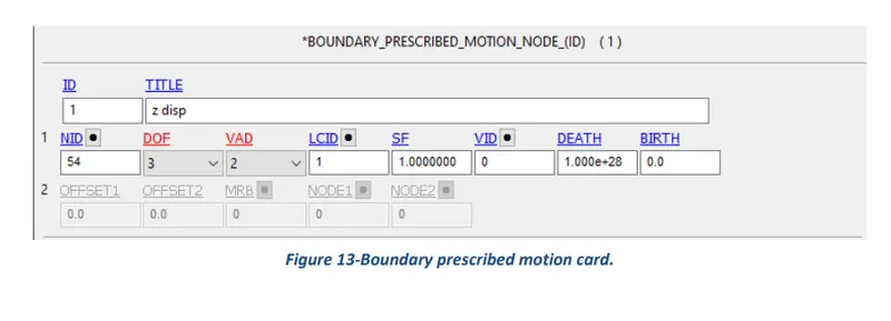
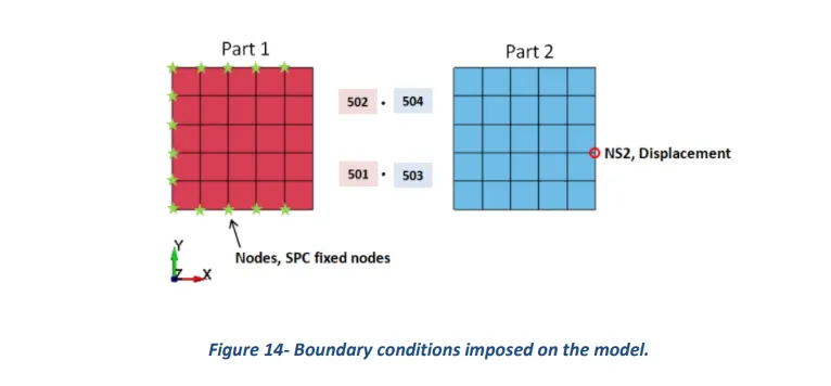
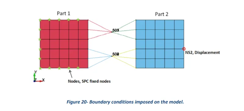
• To make this revolute joint few boundary conditions are essential. So, a displacement along the positive z-direction is applied to one of the nodes of part 2. This is defined by the Boundary_Prescribed_Motion keyword. The Z-translational degree of freedom was kept free b assigning DOF=3 in the keyword.

• Single point constraint was also used to fix part 1 at its position. Several nodes on the edge of part 1 were selected and assigned Boundary_SPC. Figure 14 shows the fixed nodes on part 1 and the node selected to give selected on part 2.

Step3)- Revolute Joint between 2 Deformable Parts:

• For deformable parts material was assigned using the Mat_Elastic keyword. Use appropriate values while defining material properties. Define the respective Material and Section keywords for the parts.
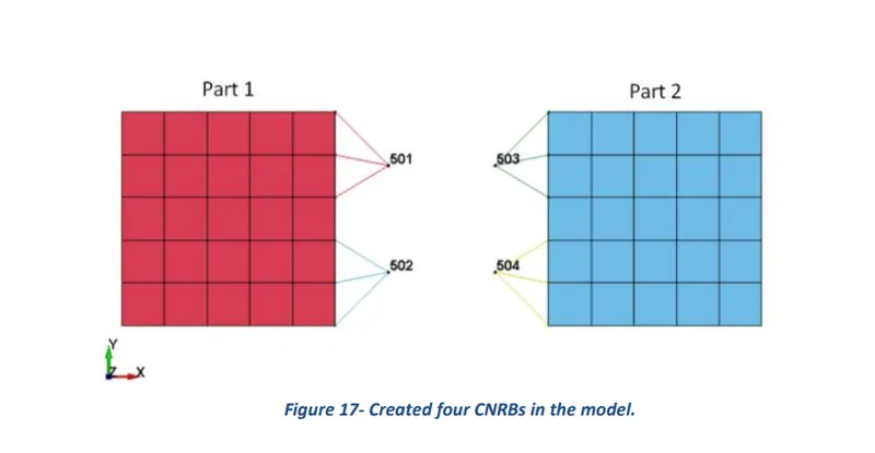
• Four nodes should be created with the help of *Constained_Nodal_Rigid_Body (CNRB) when needed to model a revolute joint between two deformable bodies.
• At first, create separate four nodes which would be used to create CNRBs. Create nodes by Element Tools>Node Editing option and give distinct IDs to all four nodes such as 501, 502, 503, and 504.

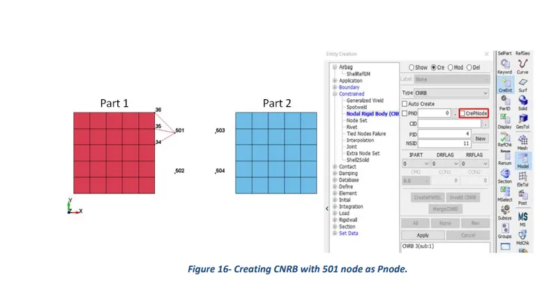
• Now go to Create Entity> Constrained Nodal Rigid Body (CNRB)> Create. Toggle off CrePNode which will disable the creation of PNODE at the center of the mass center of selected nodes. Now select the 501 node as the first point followed by 36, 35, and 34 and hit apply. A CNRB will be created with PNODE at the 501 node position.

• Similarly create a total of four CNRBs with PNODEs as 501, 502, 503, and 504. Figure 17 depicts all the four CNRBs in the model.

• According to the condition of revolute joint nodes 501 and 503 should be coincident, and similarly nodes 502 and 504 should coincide. This was achieved by Element Tools> Transform> Translate>Move option.

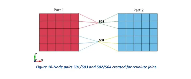
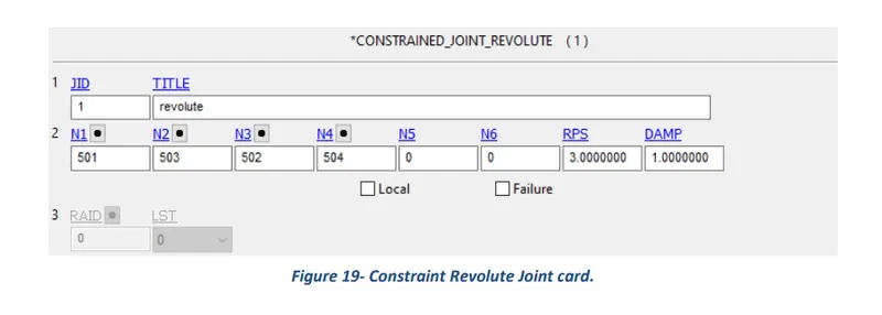
• The revolute joint was defined using the Constrained_Joint_Revolute keyword. Four nodes were defined to create a revolute joint. N1 (501) and N3 (503) nodes belong to part 1 and N2 (502) and N4 (504) belong to part 2.

• Same boundary conditions as of rigid analysis were used to fix part 1 and displace part 2 along Z-direction as discussed above.

Step 4)- The same procedure was followed to model Spherical, cylindrical, and Translational joints between two rigid and two deformable bodies as well.

4 Results

The section presents the simulation results obtained for spherical, revolute, cylindrical, and translational joints between two rigid bodies and two deformable bodies.

Simulation results of the Revolute Joint between two rigid and two deformable parts respectively.

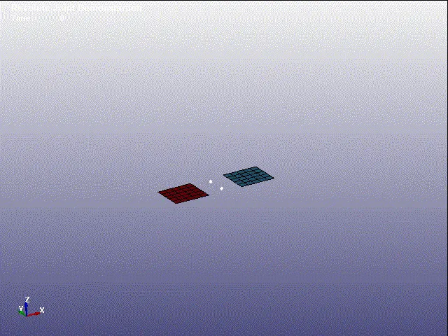
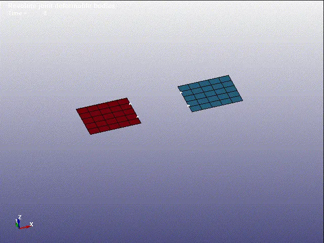
Simulation results of the Spherical Joint between two rigid and two deformable parts respectively.

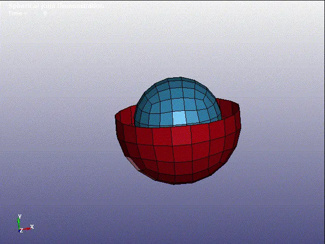
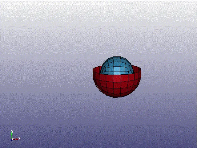
Simulation results of the Cylindrical Joint between two rigid and two deformable parts respectively.

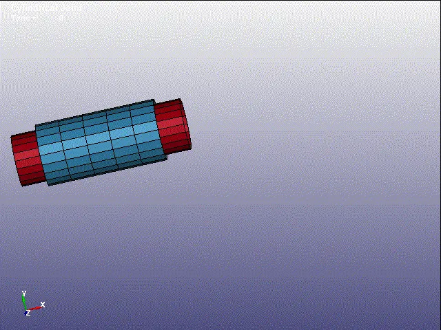
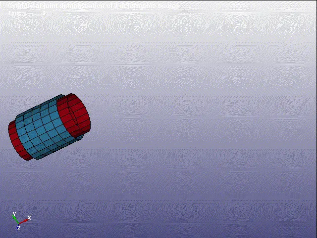
Simulation results of the Translational Joint between two rigid and two deformable parts respectively.

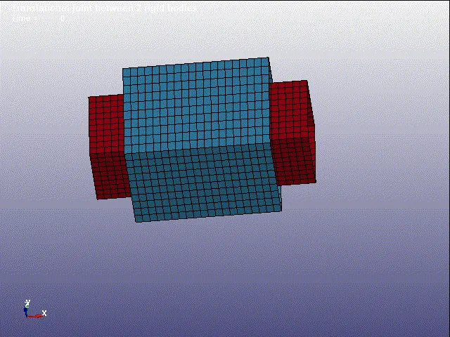
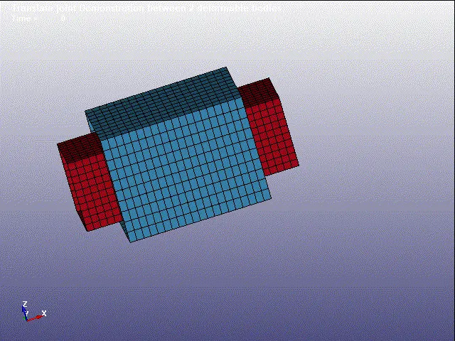
5 Conclusion

The main aim of the Week 11 challenge was to demonstrate spherical, revolute, cylindrical, and translational joints between two rigid bodies and two deformable bodies. The simulation results have presented that the constraint joints modeled behave similarly for both rigid and deformable parts.

6 Appendix

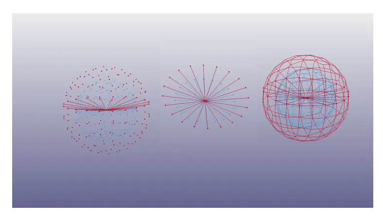
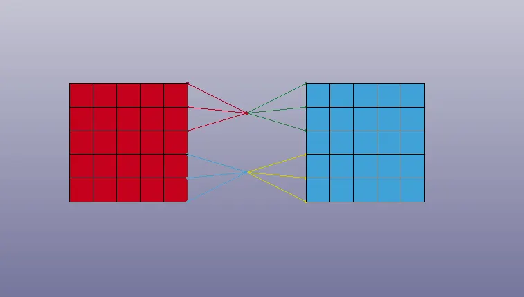
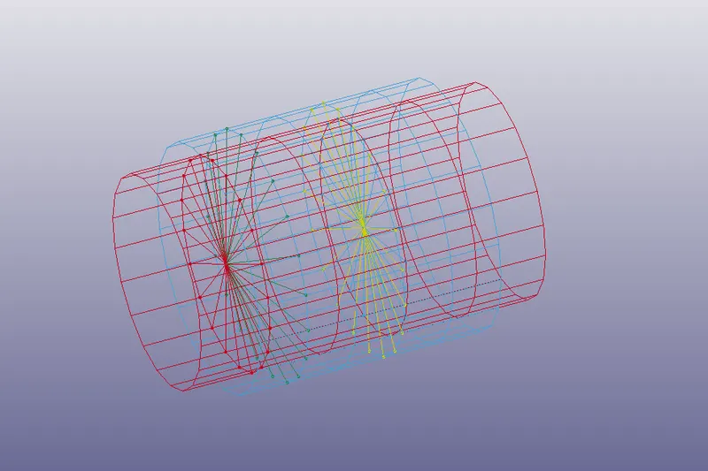
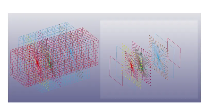
What follows hereafter is a set of images representing modeling of CNRBs at different places of deformable parts for the creation of spherical, revolute, cylindrical, and translational joints respectively.