week-11 Joint creation and Demonstration

Aim: To demonstrate spherical, revolute, cylindrical, and translational joints between two rigid bodies and two deformable bodies by using the manual for reference.

Joints

Cylindrical joint:

A cylindrical joint is a two-degrees-of-freedom kinematic pair used in mechanisms. Cylindrical joints provide single-axis sliding function as well as a single axis rotation.

Revolute joint:

A revolute joint is a one-degree-of-freedom kinematic pair used frequently in mechanisms and machines. The joint constrains the motion of two bodies to pure rotation along a common axis.

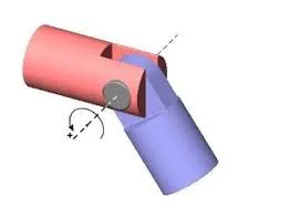
Spherical Joint:

A spherical joint, also known as a ball-and-socket joint, allows three relative rotations between the two connected segments.

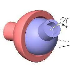
Translatory joint:

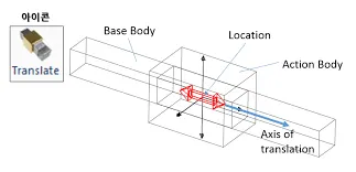
A translational joint allows one part to translate along a vector in respect of another part. The parts can only translate, not rotate, in respect of each other.

Cylindrical Joint:

This joint is derived from the rotational joint by relaxing the constraints along the centre line. This joint admits relative rotation and translation along the centreline.

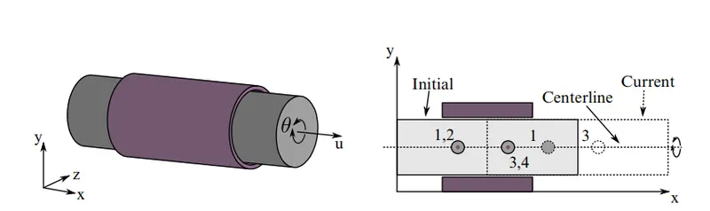
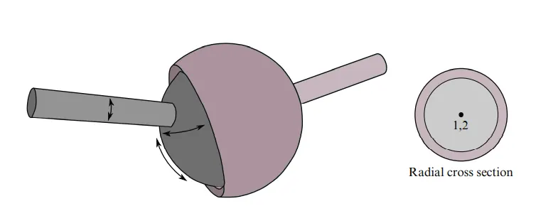
Spherical joint:

The relative motion of the rigid bodies is constrained so that nodes which are initially coincident remain coincident. In the above figure the socket’s node is not interior to the socket—LS-DYNA does not require that a rigid body’s nodes be interior to the body.

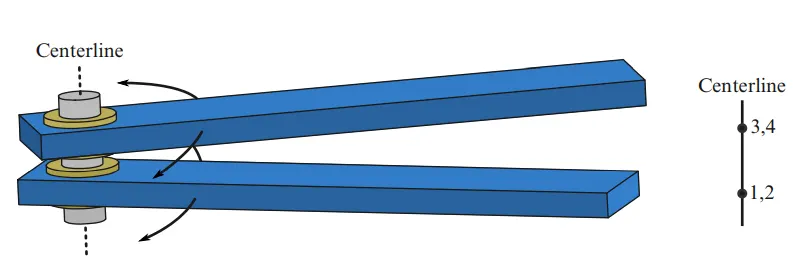
Revolute Joint:

Nodes 1 and 2 are coincident; nodes 3 and 4 are coincident. Nodes 1 and 3 belong to rigid body A; nodes 2 and 4 belong to rigid body B. The relative motion of the two rigid bodies is restricted to rotations about the axis formed by the two pairs of coincident nodes. This axis is labelled the “centreline”.

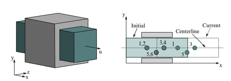
Translational joint:

This is a cylindrical joint with a third pair of off-centreline nodes which restrict rotation. Aside from translation along the centreline, the two rigid bodies are stuck together.

A joint is created using an even number of nodes, out of which every pair has the same position (XYZ coordinate). These nodes should belong to the bodies between which the joint operates.

Revolute joing using rigid bodies:

Creating geometry for the revolute joints:

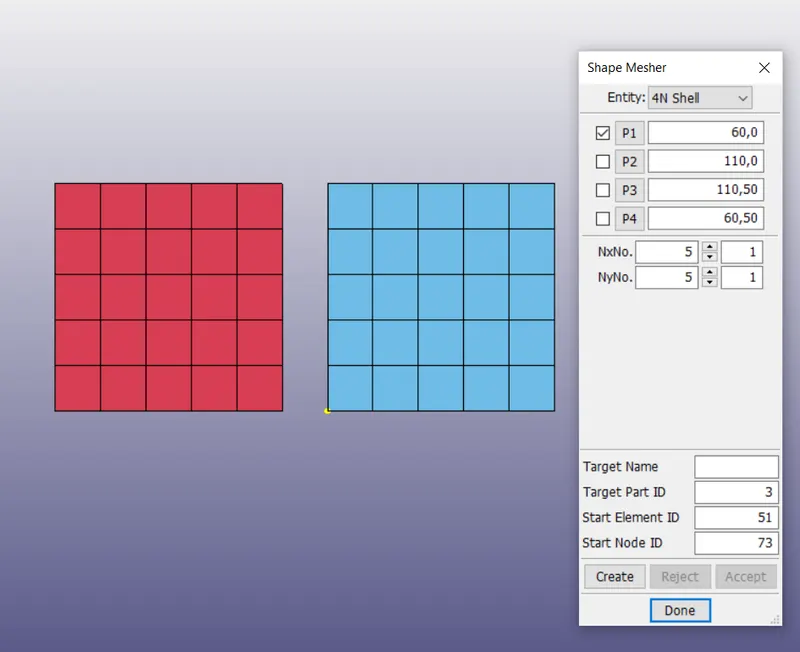
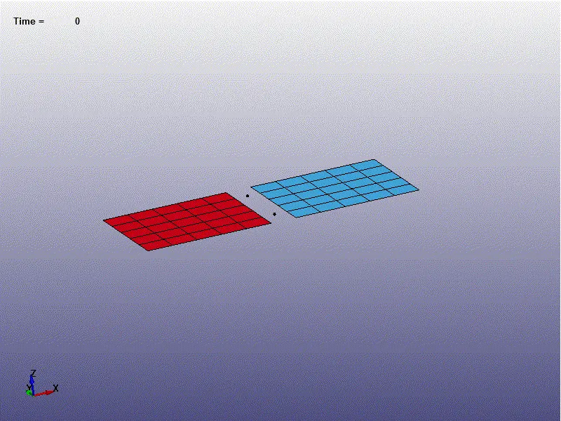
Go to shape mesher >>> 4N shell >>> provide the coordinate system as shown below.

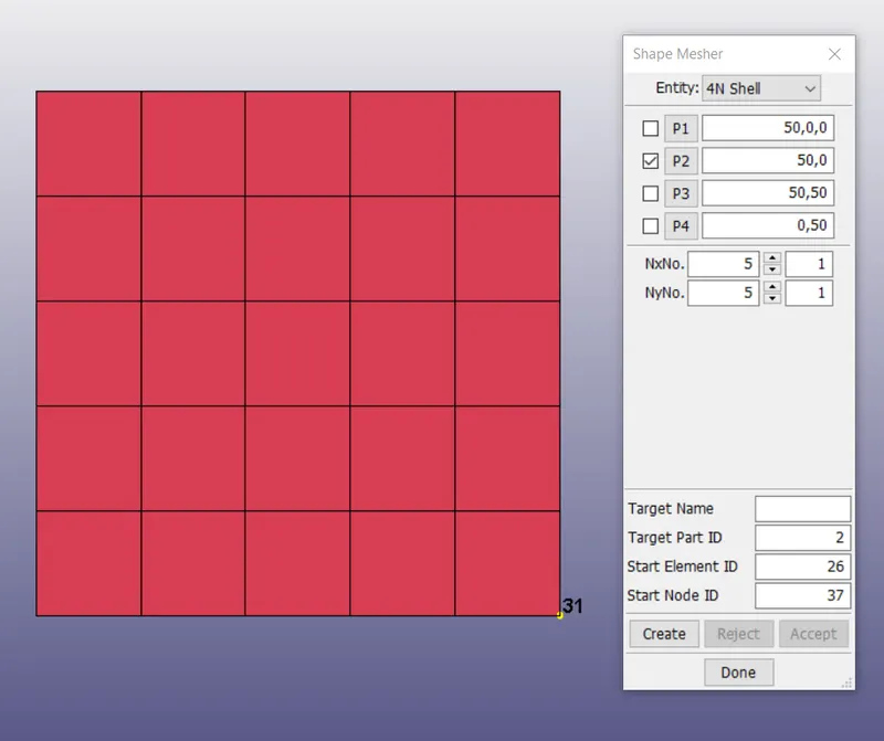
Similarly create another 4 nodes shell by providing some between two of them.

Now create two nodes in between the two shells as shown below. Provide the node ID as 101 and 102 at the same coordinates. Provide another set of nodes 104 and 104 at the same coordinates as shown below.

Node ID 101, 102 @(55,10)

Node ID 103, 104 @(55,40)

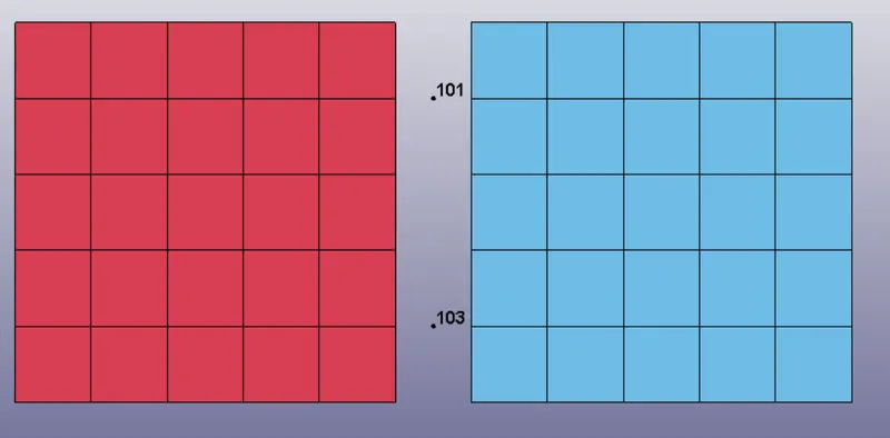
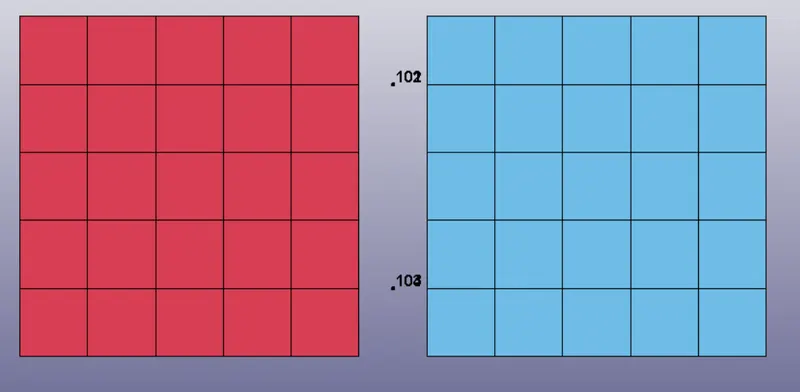
Crete a node set with ID 1 for nodes 101, 103.

Create a node set with ID 2 for nodes 102, 104.

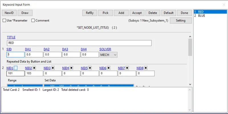
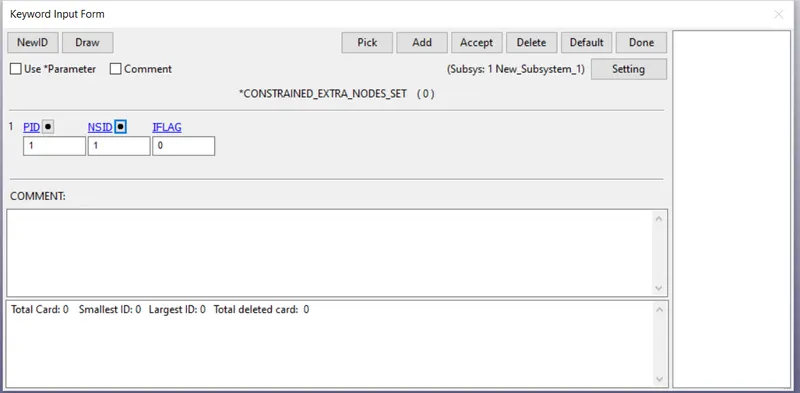
Go to keyword manager >>> Constrained >>> Constrained_Extra_nodes_set

Provide the part id and thier nodes.

We have selected the nodes 101 and 103 of node set ID 1 to belong to the part set ID 1.

We have selected the nodes 102 and 104 of node set ID 2 to belong to the part set ID 2.

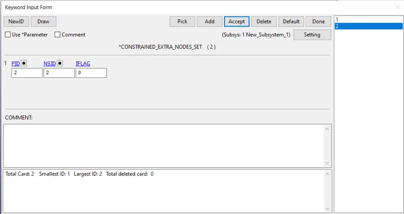
Now we have to define a joint between the nodes created.

Now we can see the nodes 101, 103 belongs to part 1, nodes 102, 104 belongs to part 2.

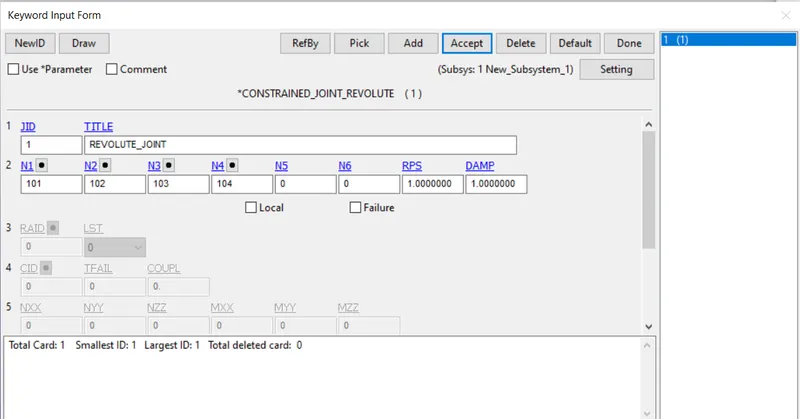
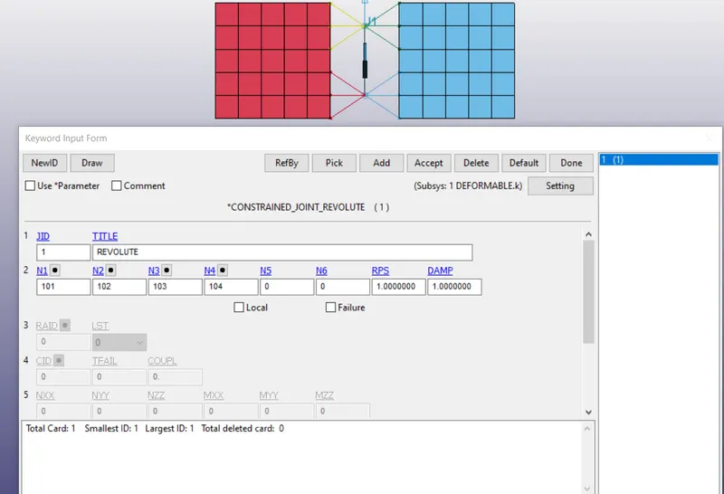
Create Constrained_joint_revolute card and provide the N1, N2, N3, N4.

Select N1 as node belonging to part 1

Select N2 as node belonging to part 2

Select N3 as node belonging to part 1

Select N4 as node belonging to part 2

Provide the boundary conditions such that the red part is constrained in all the directions.

Provide the prescribed motion to the blue part in z direction to get the revolute motion.

All the nodes of the red part is constrained.

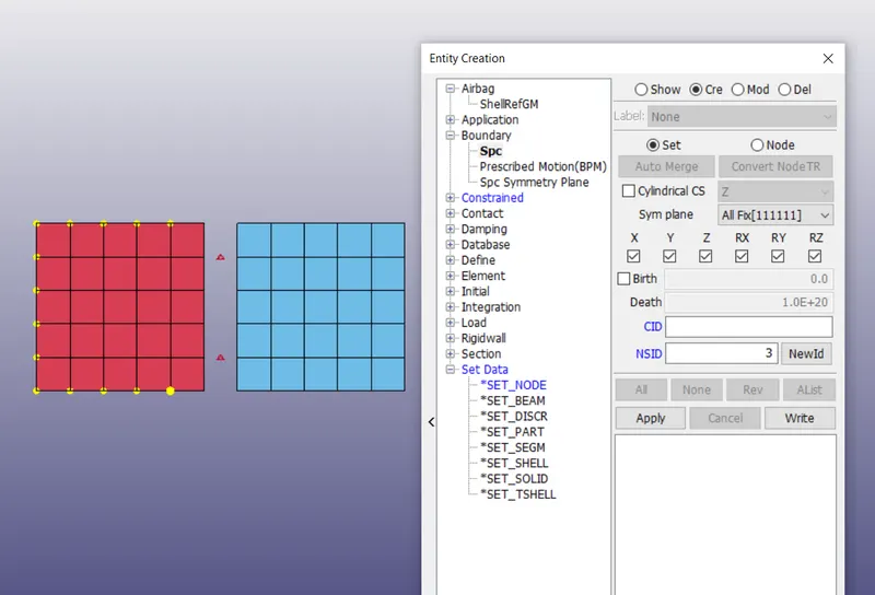
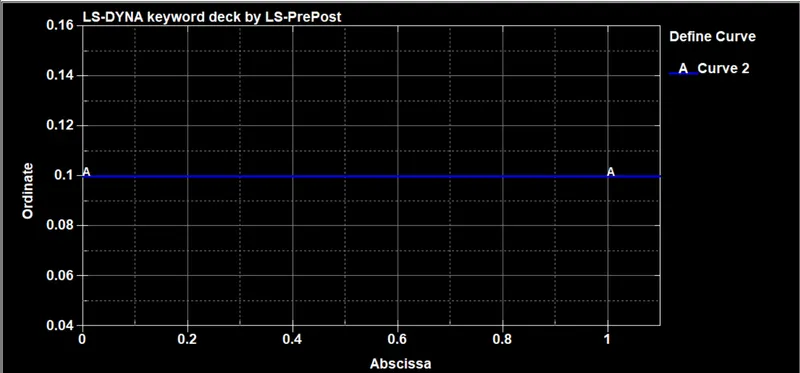
To define the displacement to the blue part. Create a curve which defines how the displacement is taking over the time.

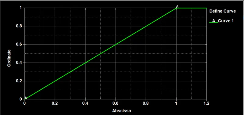
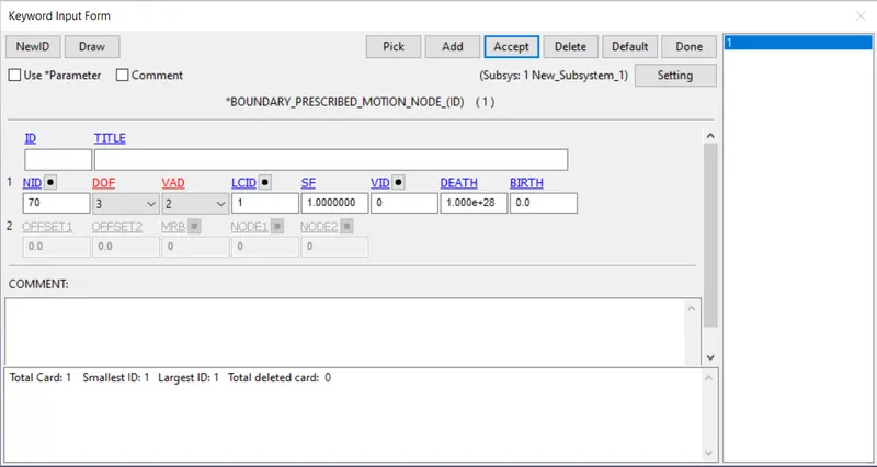
We have to create the boundary_prescribed_motion_node.

Provide the DOF as 3 representing the motion is applied in z direction.

VAD is representing the displacement is the motion that is prescribed.

Provide the LCID of the curve that is created.

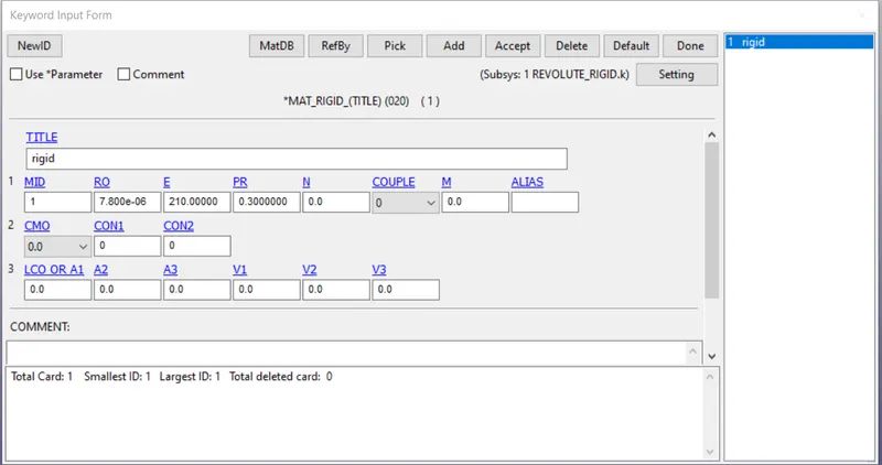
Create the material card:

Mat_rigid is created as shown below.

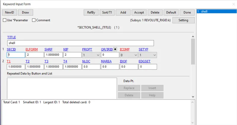
Create the section card.

As the created parts are shell. Create section_shell.

Provide ELFORM = 2 and thickness of the shell as 1mm.

Create the control cards to define how run is taking place whether implicit or explicit.

Control_implicit_auto is created.

IAUTO = 0 represents the constant time step size.

IAUTO = 1 represents the Automatic adjustion of the time step

ITEOPT is the average number of iterations

ITEWIN is the tolerance value

In this case ITEOPT = 100, ITEWIN = 50

It is representing that, if number of interations is in between 50 (100-50) and 150 (100+50) the time step is going to remain constant.

If less than 50, the time step is increased and if more than 150, the time step is decreased.

In our case, the Automatic adjustion of the time step takes place by using the above data as IAUTO = 1.

IMFLAG = 1 is activating the implicit solver.

Implicit_Solver is represnting the linear solver.

Implicit_Solution represents the non-linear solver.

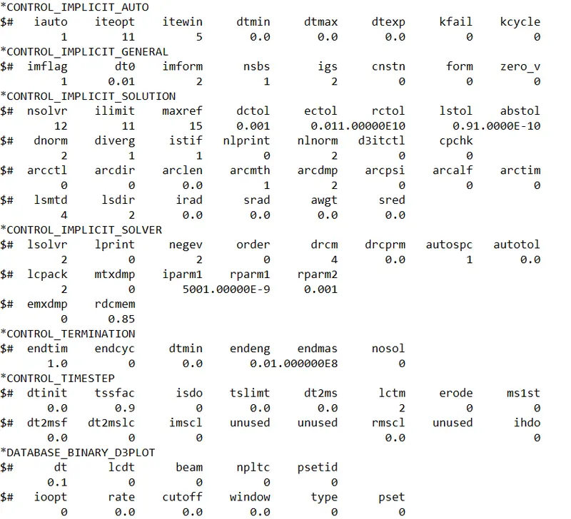
Control_Termination:

The run time of the simulation is given as 1ms.

Create the database card:

Request for D3PLOT:

DT = 0.1 :Time interval at which the animation files should be printed.

*DATABASE_EXTENT_BINARY Flag for output of strain tensors.

Writes strain tensor data to d3plot and elout.
For shell and thick shell elements two tensors are written, one at the innermost and one at the outermost integration point. For solid elements a single strain tensor is written.

Requesting the outputs:

In Database_Ascii >>> Activate GLSTAT, ELOUT, RCFORC

GLSTAT: GLOBAL DATA

ELOUT: ELEMENT DATA

RCFORC: Resultant Internal forces.

The control timestep card is defined to show how timestep is varying over the time.

ANIMATION OF REVOLUTE JOINT

REVOLUTE JOINT BETWEEN TWO DEFORMABLE BODIES:

Create two shells by using the same procedure and create 4 nodes at 4 different locations to define the constrained nodal rigid body at the individual node.

The nodes are created at points as shown below.

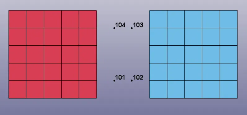
Create CNRB's:

Go to Model and Part >>> Constrained >>> Nodal rigid body >>> Disable the CrePNode as shown below >>> Select one created node >>> Then select the nodes from corner of the near of part as shown below >>> Apply.

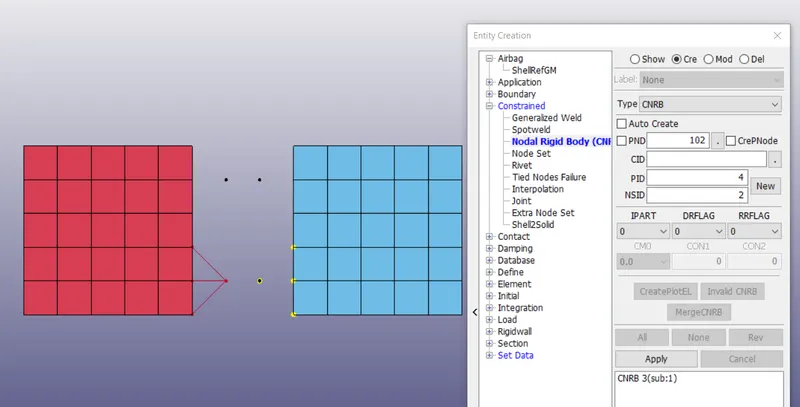
Similarly, Do the same for the 4 nodes.

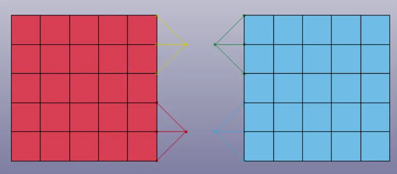
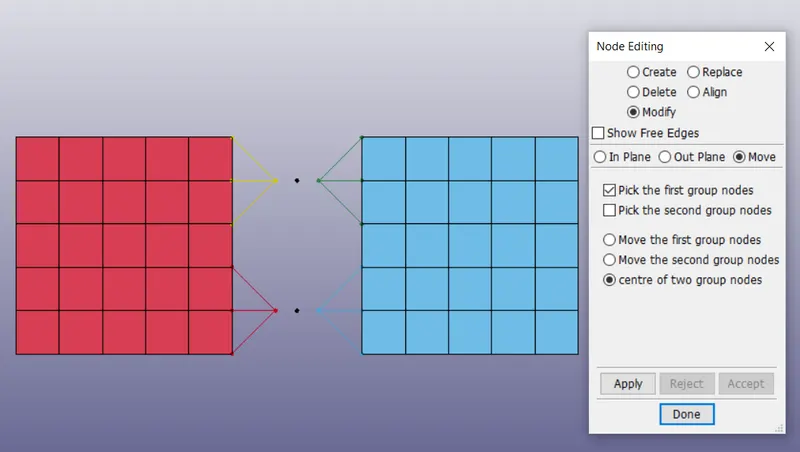
Go to Element and mesh >>> Node editing >>> Modify >>> Move >>> enable center of two group nodes >>> pick first group node >>> Pick second group node >>> Apply >>> accept >>> Done.

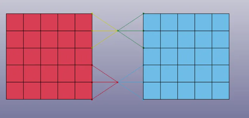
GUI doest get updated as soon as you create, Save the file and open it again.

The Coincident of the respective nodes is shown below.

Go to Constrained_Joint_Revolute and select the nodes N1, N2, N3, N4 as explained earlier.

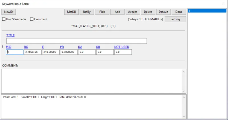
Create the elastic material card:

Create the section card, Boundary conditions, Control card, Database card as explained earlier and run the simulation.

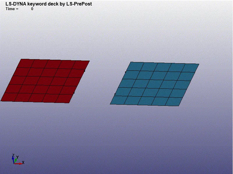
The Simulation of deformable revolute joint is shown below:

CYLINDRICAL JOINT__RIGID:

Creating geometry for the Cylidrical joints:

Go to shape mesher >>> 4N shell >>> provide the coordinate system as shown below.

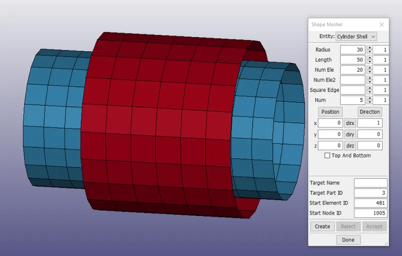
Now create 2 ends @ center of the either sides of the outer part.

NODE ID 1001, 1002 at one end

NODE ID 1003, 1004 at the other end.

Now,

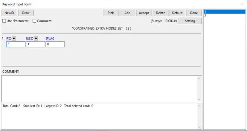
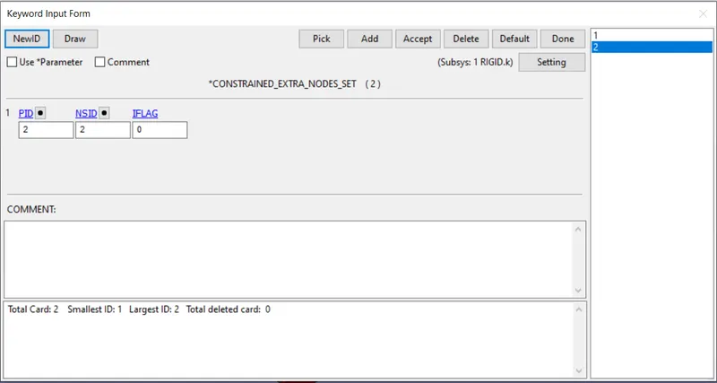
Go to keyword manager >>> Constrained >>> Constrained_Extra_nodes_set

Provide the part id and thier nodes.

We have selected the nodes 101 and 103 of node set ID 1 to belong to the part set ID 1.

We have selected the nodes 102 and 104 of node set ID 2 to belong to the part set ID 2.

Now we have to define a joint between the nodes created.

Now we can see the nodes 101, 103 belongs to part 1, nodes 102, 104 belongs to part 2.

Create Constrained_joint_Cylidrical card and provide the N1, N2, N3, N4.

Select N1 as node belonging to part 1

Select N2 as node belonging to part 2

Select N3 as node belonging to part 1

Select N4 as node belonging to part 2

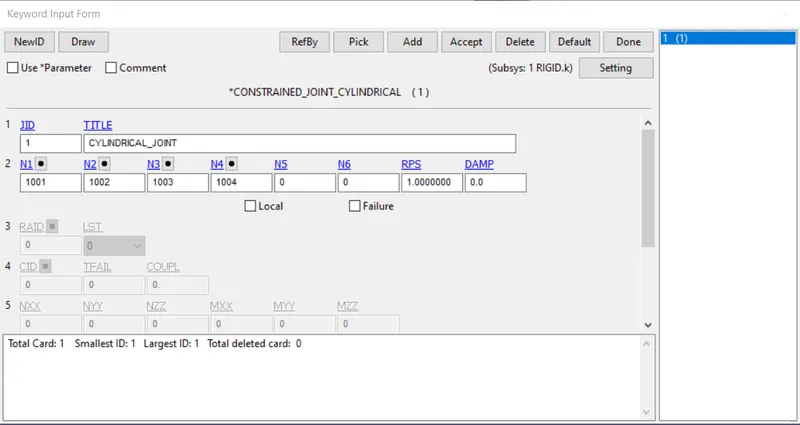
We can see the Cylindrical joint is created:

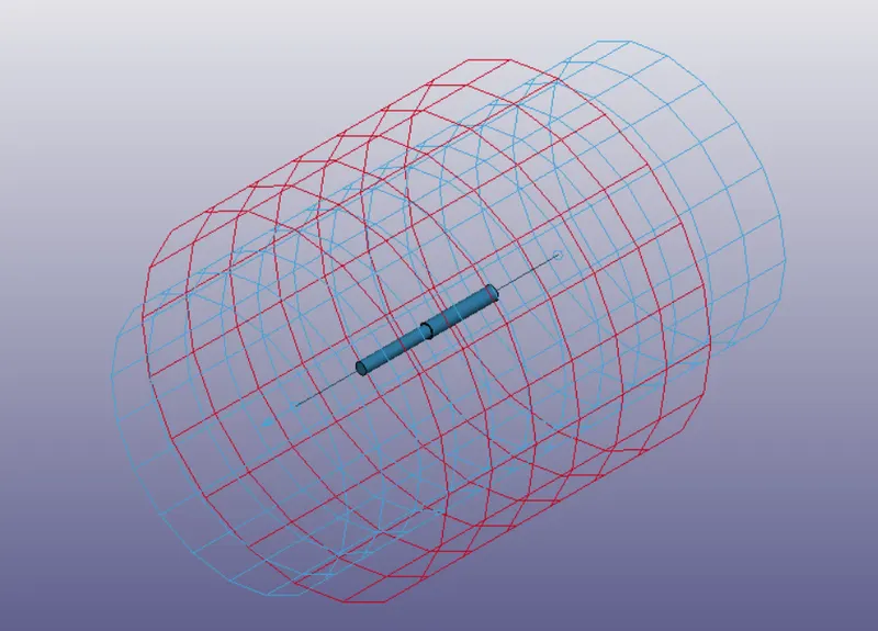
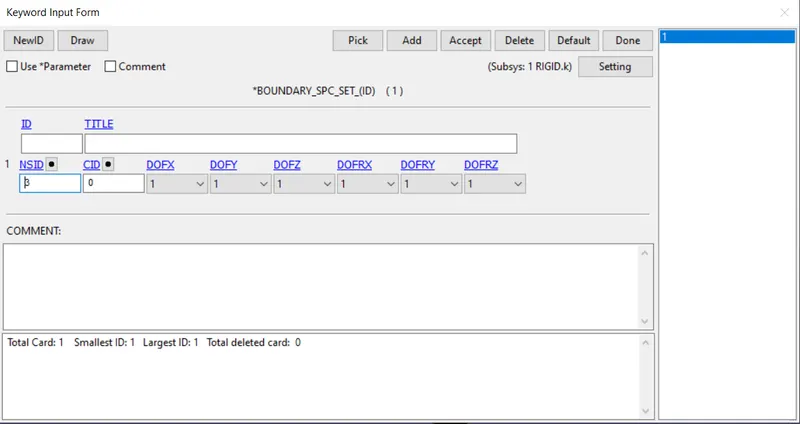
We have to constrain all DOF of the outer part

We have to provide the velocity_rigid to the inner part to see the motion of cylindrical joint.

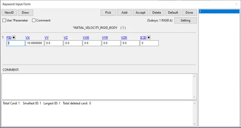
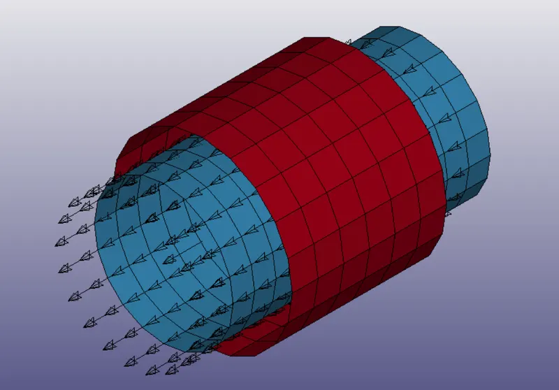
The applied velocity is shown below:

Create the section card, Boundary conditions, Control card, Database card as explained earlier and run the simulation.

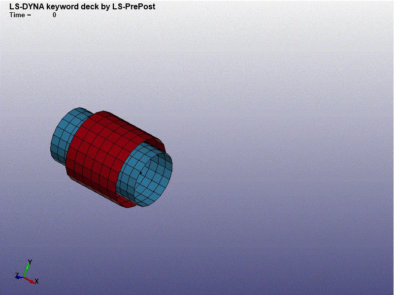
The Simulation of deformable cylindrical joint is shown below:

CYLINDRICAL JOINT__DEFORMABLE:

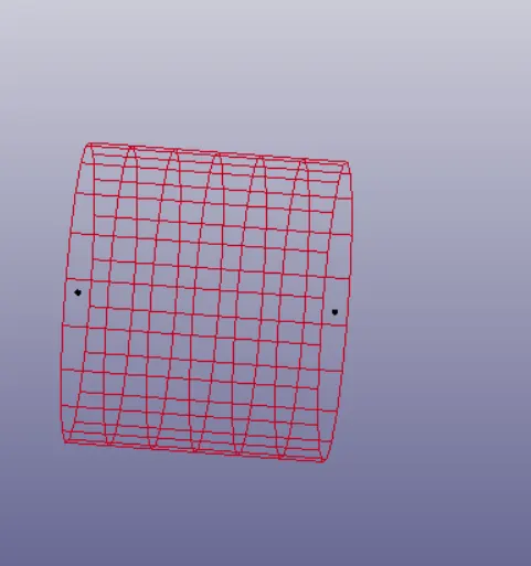
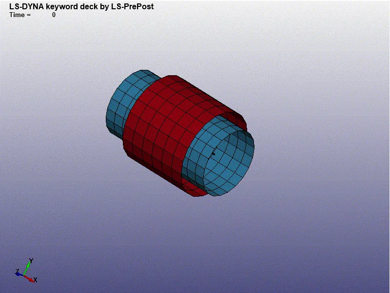
Create the cylider_shell in the shape mesher as discussed earlier.

Create two pair of nodes at the either side ends of the cylinder.

Create CNRB's by selecting the outer nodes of the respective ends.

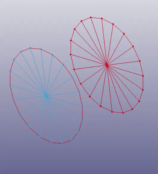
Similarly, create CNRB's to the inner cylinder by selecting the other pair of nodes on the either sides.

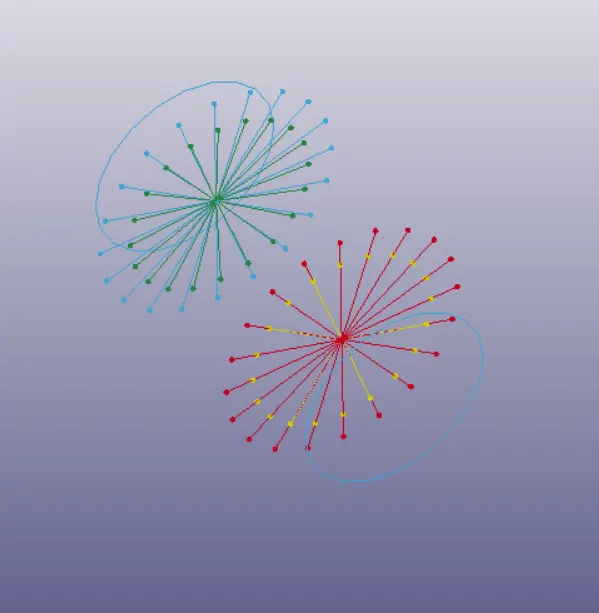
Now Go to Constrained_Joint_cylindrical is craeted as shown below:

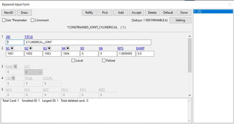
The cylindrical joint is created:

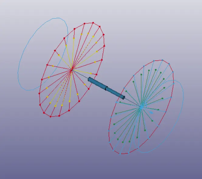
The material created is a elastic material.

Create the section card, Boundary conditions, Control card, Database card as explained earlier and run the simulation.

The simulation of cylindrical joint_Deformable:

SPHERICAL_JOINT_RIGID:

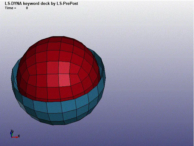
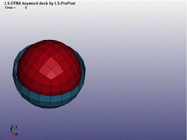
Go to Mesh >>> Shape Mesher >>> Spherical shell >>> create two parts with two different diameter.

The half part of the outer sphere is deleted as shown below.

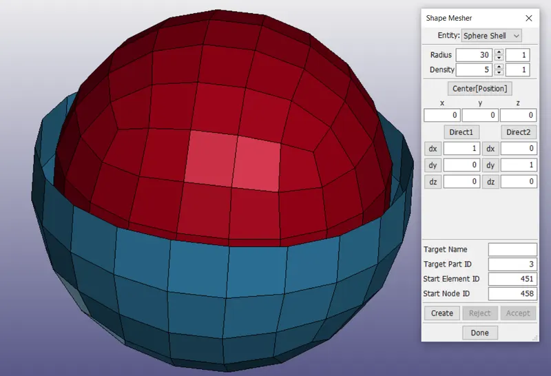
Two nodes at creeated at the center representing with ID 456, 457.

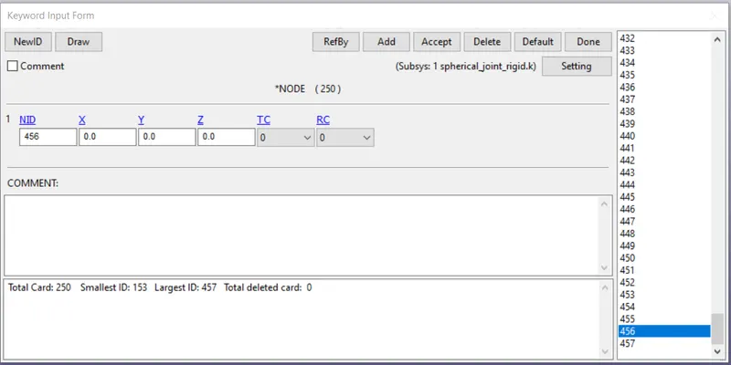
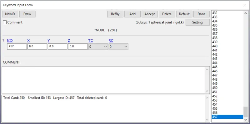
Go to Constrained_Extra_nodes and select one node for one part.

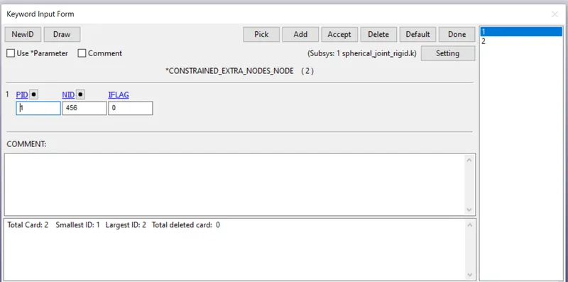
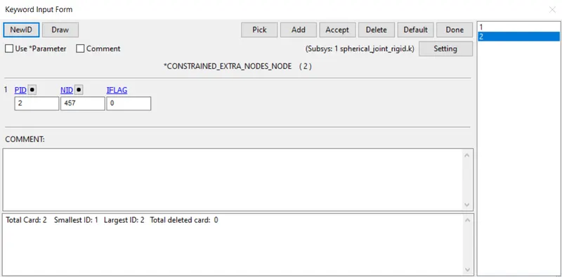
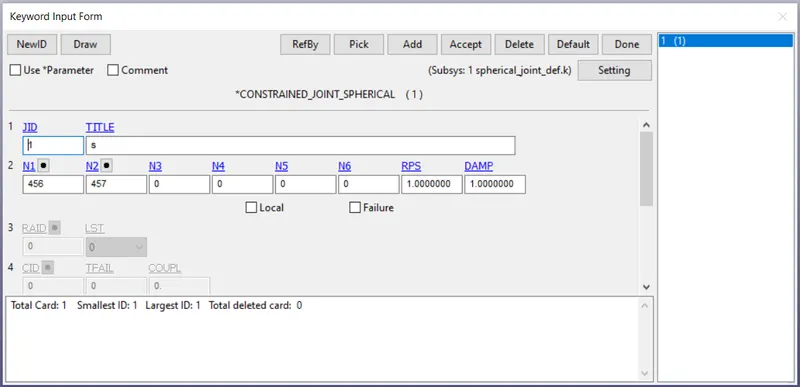
Go to Constrained_Joint_Spherical and select N1 for part1 and N2 for part 2.

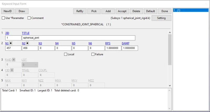
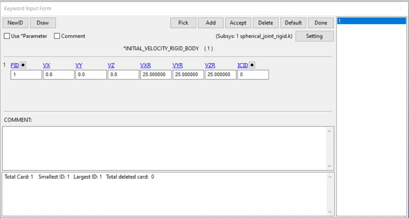
Provide the velocity to the inner part.

As this is a spherical joint, we have to provide the Rotary motion.

The material created is a MAT20 rigid material.

Create the section card, Boundary conditions, Control card, Database card as explained earlier and run the simulation.

The simulation of spherical_Joint_Rigid:

SPHERICAL_JOINT_DEFORMABLE:

Similarly create two parts as discussed, and create a pair of nodes at (0, 0, 0).

Go to Create entity >>> Constrained >>> Nodal rigid body >>> Disable the CrePNode as shown below >>> Select one created node >>> Then select the nodes from corner nodes of the one part as shown below >>> Apply.

Similarly do it again for the other part using the other created node.

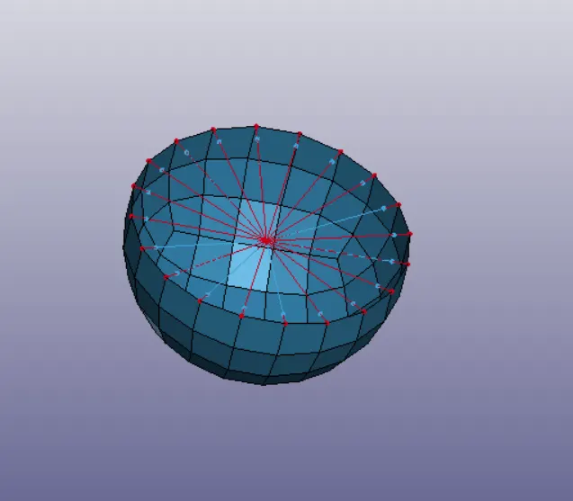
create the Constrained_joint_Spherical and select the nodes that are initially created.

The CNRB"s created:

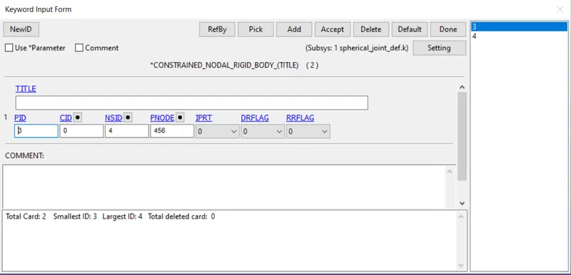
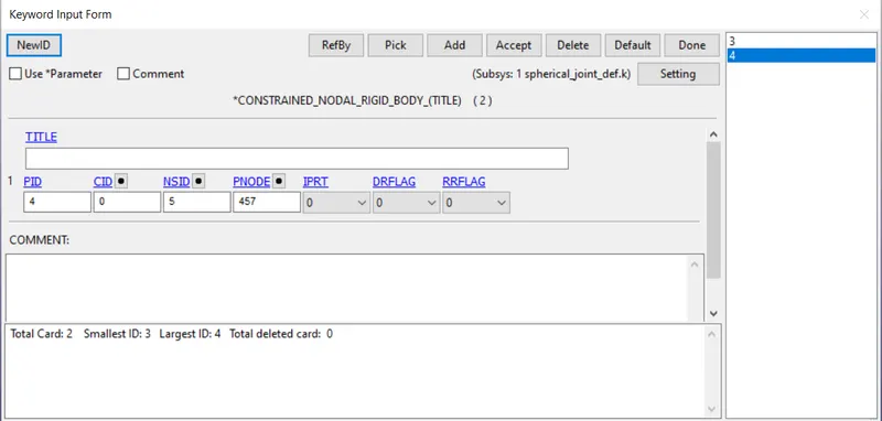
The material created is a MAT01 elastic material.

Create the section card, Boundary conditions, Control card, Database card as explained earlier and run the simulation.

The simulation of spherical_Joint_Deformable:

Translatory Joint Rigid:

Create the Box shell and delete the faces on one side. Create the smaller part to see the translation motion.

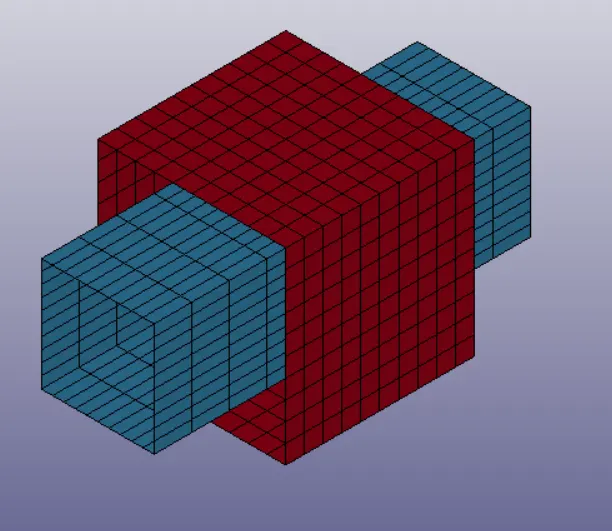
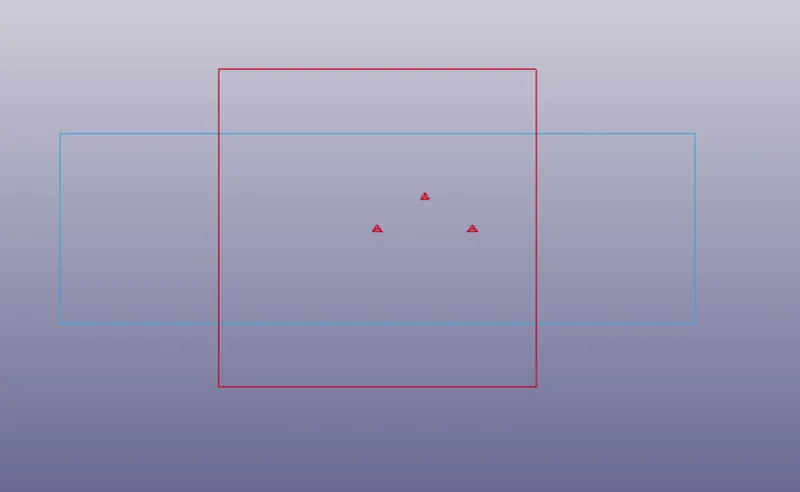
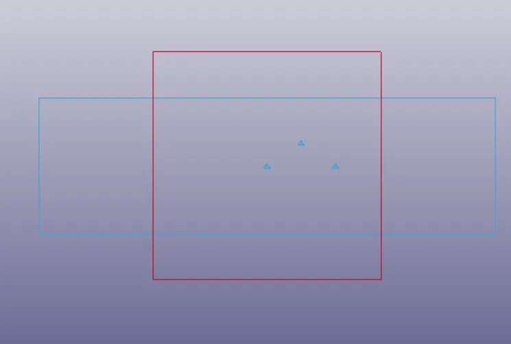
Three pairs of nodes are created such a way that two pairs are collinear and in the center line and the other pair is offsetted from the center line and is parallel.

We can see where nodes are created from the top view.

The red nodes created belong to outer part.

The blue nodes created belong to inner part.

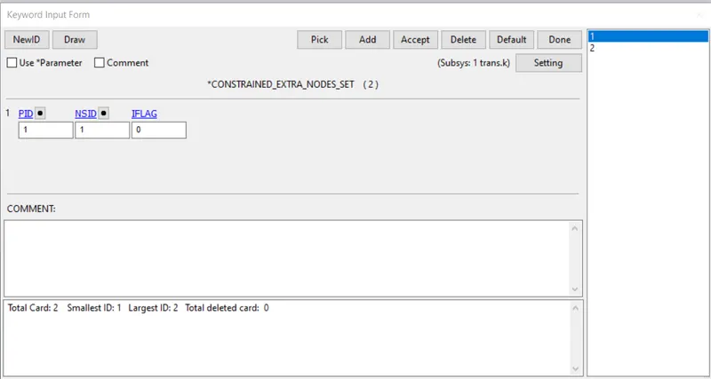
Constrained_Node_set is created by selecting the nodes belonging to PID 1

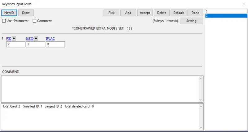
Constrained_Node_set is created by selecting the nodes belonging to PID 2

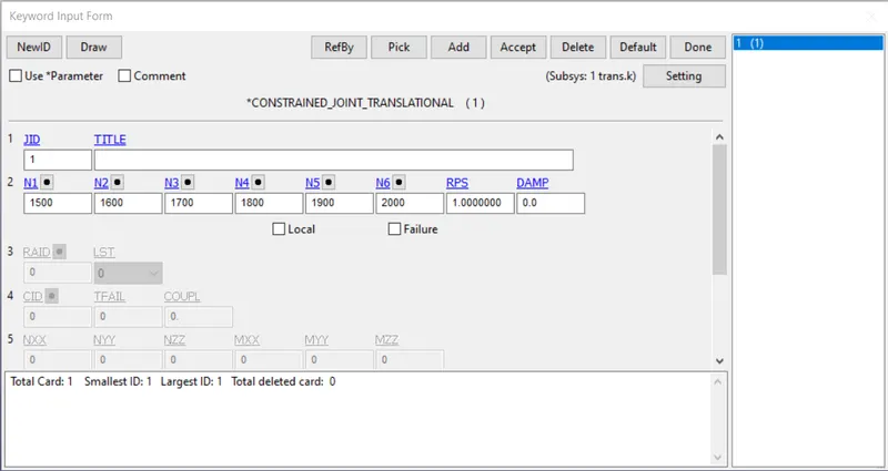
Create the Constrained_Joint_Translational card to define the joint.

Select N1 as node belonging to part 1

Select N2 as node belonging to part 2

Select N3 as node belonging to part 1

Select N4 as node belonging to part 2

Select N5 as node belonging to part 1

Select N6 as node belonging to part 2

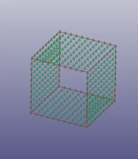
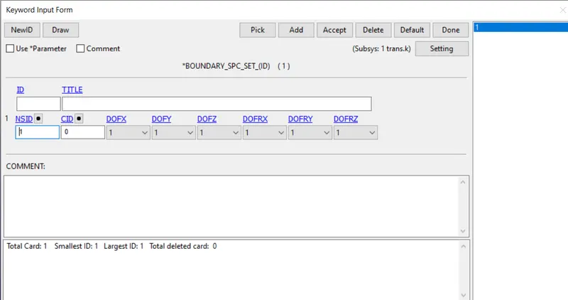
the outer part is constrained in all degrees of freedom:

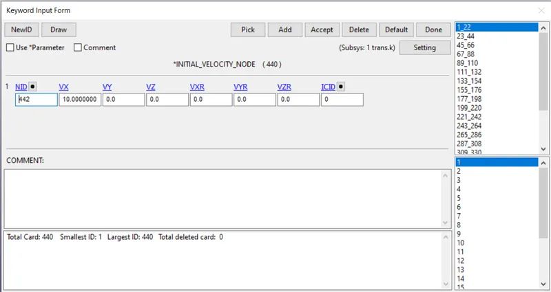
The initial velocity is provided to the inner part.

Vx = 10 mm/ms

The material created is a elastic material.

Create the section card, Boundary conditions, Control card, Database card as explained earlier and run the simulation.

Animation of Translatory_Joint_Rigid:

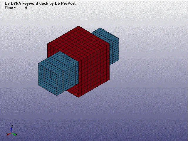
Translatory Joint__Deformable:

Create the Box shell and delete the faces on one side. Create the smaller part to see the translation motion.

Three pairs of nodes are created such a way that two pairs are collinear and in the center line and the other pair is offsetted from the center line and is parallel.

We can see where nodes are created from the top view.

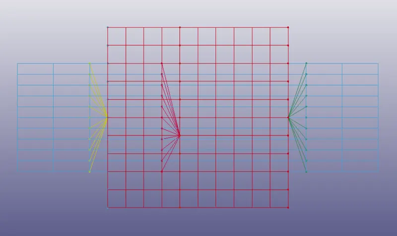
We can see how nodes are offsetted from the front view:

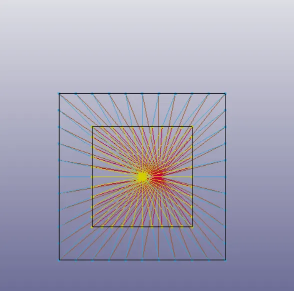
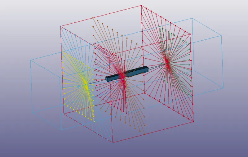
The CNRB's that are created:

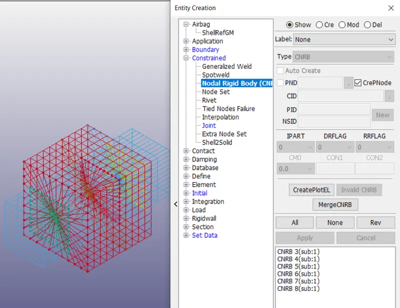
We can see there are six CNRB's that are created.

Create the Constrained_Joint_Translational card to define the joint.

Select N1 as node belonging to part 1

Select N2 as node belonging to part 2

Select N3 as node belonging to part 1

Select N4 as node belonging to part 2

Select N5 as node belonging to part 1

Select N6 as node belonging to part 2

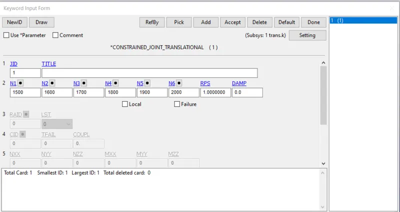
The translatory joint that is created is shown below

The outer part shoulb be constrained in all degrees of freedom.

The initial velocity is provided to the inner part.

Vx = 10 mm/ms

The material created is a elastic material.

Create the section card, Boundary conditions, Control card, Database card as explained earlier and run the simulation.

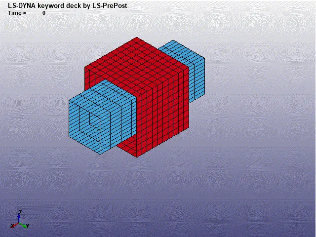
Animation of Translatory_Joint_Deformable:

Conclusion:

• All the given joints are modeled for rigid and deformable bodies.
• Revolute Joint: Two pair of nodes are to be defined, which are coincident to each other. Only rotation happens between to points using revolute joint
• Cylindrical Joint: two pairs of nodes on either ends of cylinder on the central axis. Both translation and rotation are possible by using this joint.
• Spherical Joint: two nodes are defined at the center. Only rotational degree of freedom is possible in spherical joint.
• Translatory joint: 3 pairs of nodes are to be defined. 2 pairs are defined along the central axis on either ends of shell, 1 pair offsetted from the central line but parallel to the other node pairs. Only translation is possible using this joint. The off-setted nodes restrict the rotary motion.
• *CONSTRAINED_EXTRA_NODES and *CONSTRAINED_NODAL_RIGID_BODY are used to create joints between rigid and deformable bodies respectively.