week-11 Joint creation and Demonstration

Joint creation and Demonstration:

Aim: Joint creation for rigid and deformable bodies

Types of joint:

Revolute joint:

Steps followed:

All units taken here are in kg mm ms.

Case 1: REVOLUTE JOINT FOR RIGID BODIES:

Meshing:

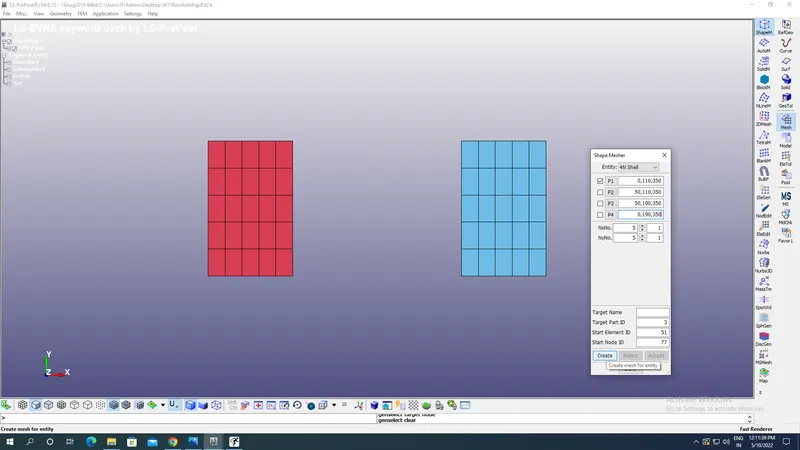
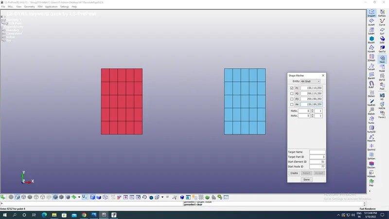
First open the LS Prepost go to mesh option under which go to Shape mesher with 4N Shell with appropriate coordinates for both the red & blue shell elements as shown in the image below:

Nodes creation:

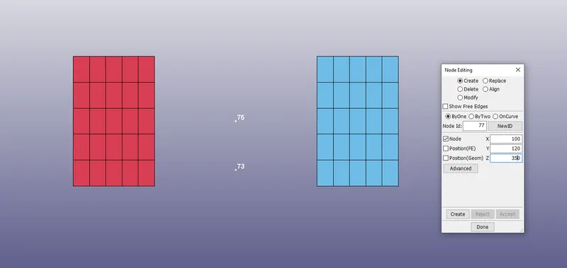
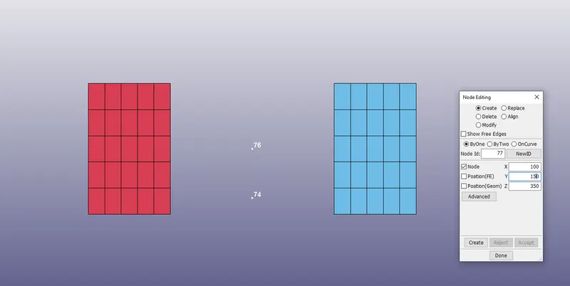
Now create the 4 nodes with similar coordinates for the two like with Node IDs 73,74 with coodinates 100,120,350 while coordinates of node with Ids 75 & 76 is 100,150,350 under Element Tool-Node edit option in the Toolbar at the extreme left side as shown in the image below:

Section:

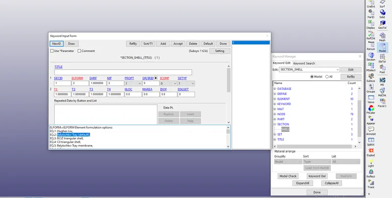
Now create a section shell under Models-Keyword-Section-Shell option as shown in the image below with proper section ID,element formulation as 2 for Belytschko-Tsay formualtion and shell thickness of 1 mm:

Material:

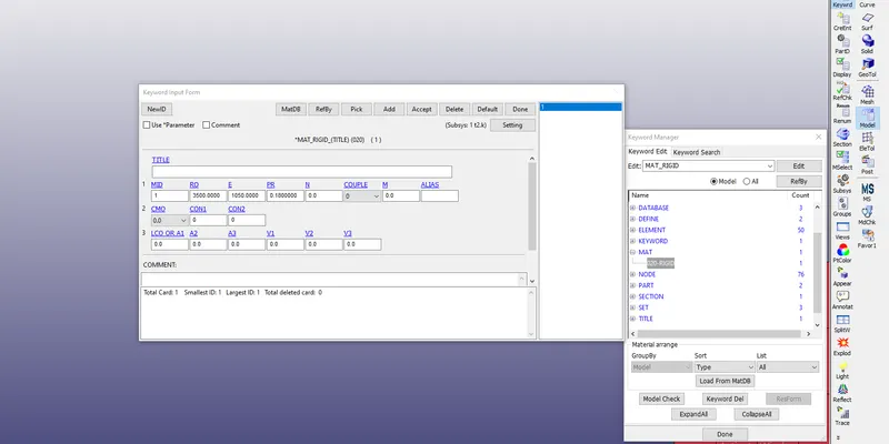
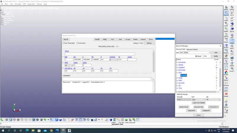
Now select the MAT card under Keyword option with MAT_020_RIGID with properties of one of the most rigid material of Diamond with density 3500 kg/ mm^3,Young's Modulus 1050 GPa & Possion's Ratio as 0.18 with appropriate material ID:

PARTS:

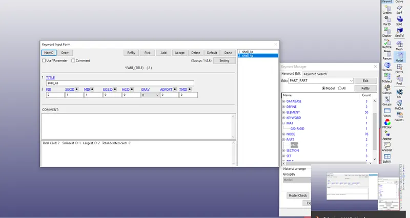
Now assign part ID under parts Keyword by assigning appropriate section and material IDs created before for both the shell parts under keyword option:

Set Creation:

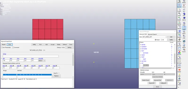
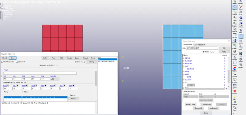
Now create two sets with node Ids of 73 & 75 and 75 & 76 as shown in the image below with proper Set IDs:

Constrained:

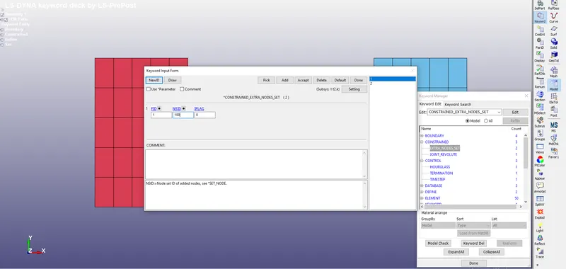
Now apply the constrained under Keyword option with Extra nodes sets option by selecting the IDs of node set which we prepared in previous steps.This extra node set is assumed to be the part of rigid body but can even be outside the rigid body.This option is manily used for placing joints between any two rigid bodies.

The part Ids of 2 parts are selectedc with proper node set Ids as shown in the image below:

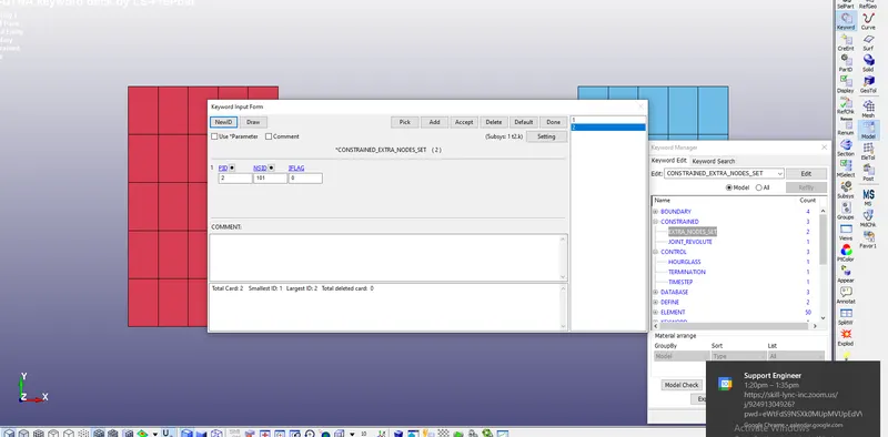
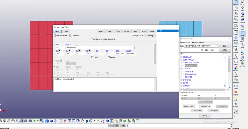
Now apply the Constrained Joint Revolute option with proper node selction for Body A and B having nodes side by side:

Boundary Canditions:

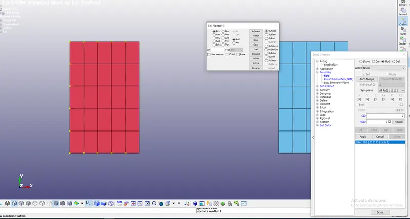
Now apply boundary canditions among which one is Single point Constrained applied to fix the one of two shell body by selecting proper nodes as shown in the image below:

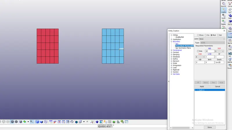
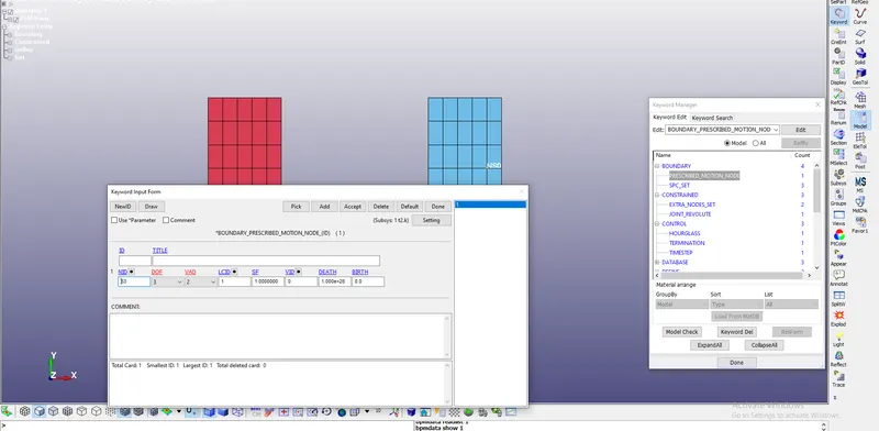
Now apply Prescribed Rigid Motion Node with dof=3 i.e. translational motion along Z axis with Displacement in accordance with LCID.\

Curves:

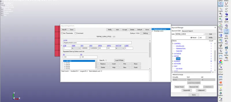
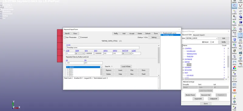
Go to define option under Keyword and apply the curve by Insert option for both Displacement and time steps as shown in the image below:\

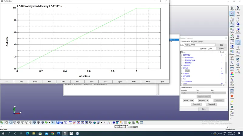
Displacement vs Time plot with scale factor of 10 along ordinates i.e Displacement:

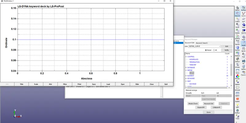
Timestep curve plot:

Controls:

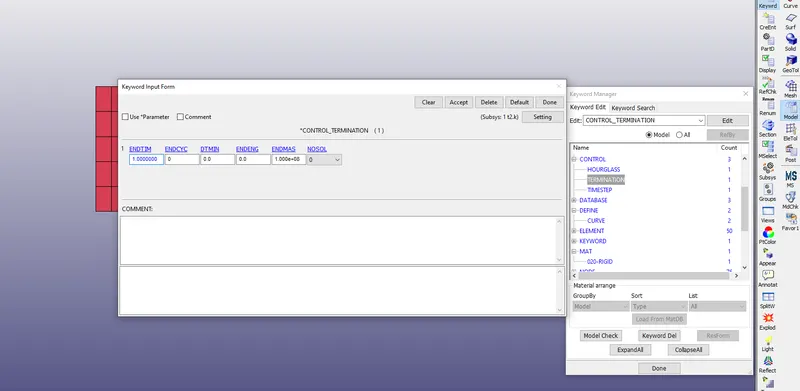
Termination: This is provided to stop the simulation after the animation with appropriate End Time as 1 ms as shown below:

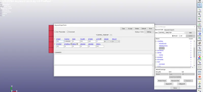
Timestep: This card is provided manily with rigid bodies to set structural time step size during solutions elementwise with LCTM assigned with Timestep curve as shown in the image below:

Output requests:

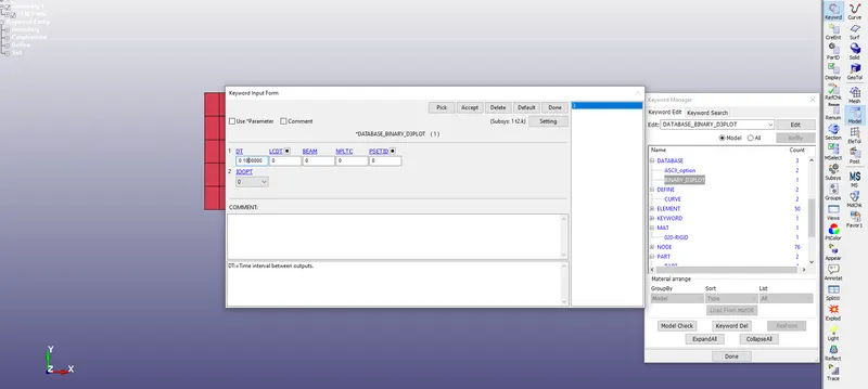
Go to Database under Keyword option with Binary d3plot with time interval between outputs as DT=0.01ms

Now save the files at appropriate location and try running it in under File-Run as LS DYNA option.

RESULTS:

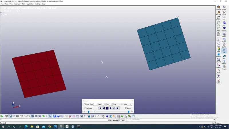
Binary d3 Plot appears of revolute Joint with rigid bodies as shown in the image below:

Case 2:

Revolute Joint with Deformable bodies:

Materials:

Under Mat option under keyword take 001 MAT_Elastic with material parameters as shown in the image below so that body here can be capable of deformation as shown in the image below:

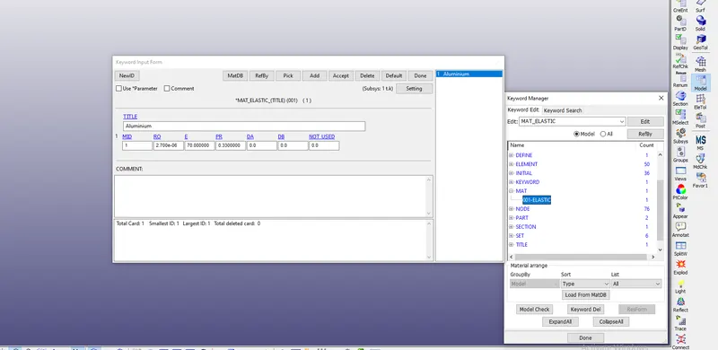
All meshes,parts,sections & Boundary SPC remains same as above only .

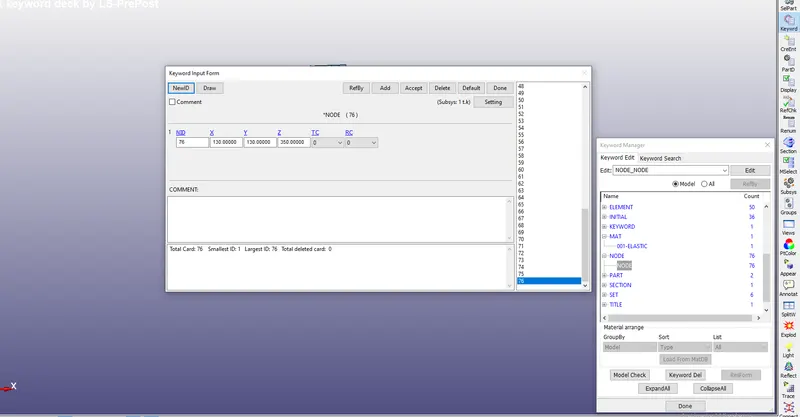
Now create four different nodes with different coordinates:

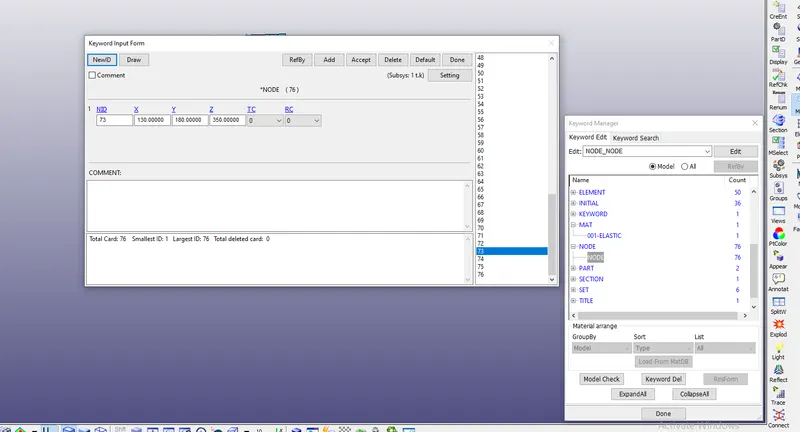
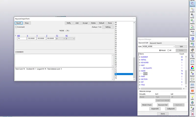
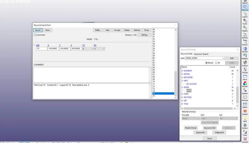
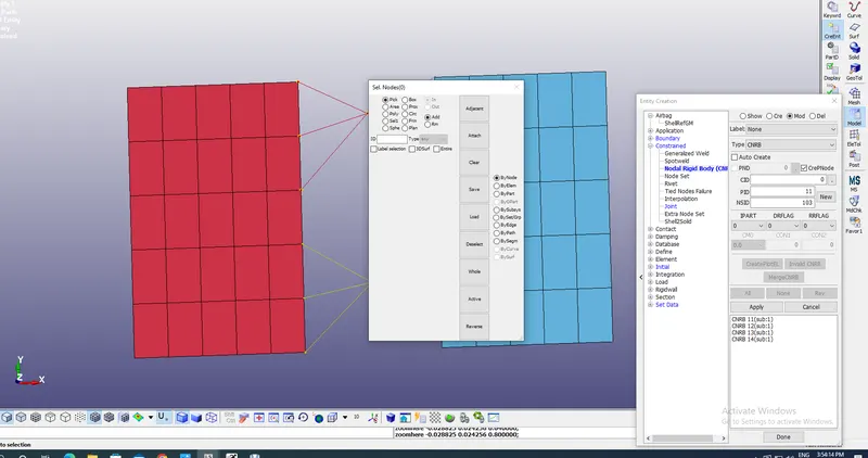
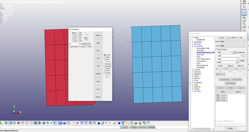
Now apply Constrained Nodal Rigid bodies with each node conneting 3 of its adjacent nodes.

Constrained Nodal rigid body is used to apply rigid nodes at the joints within deformable bodies to make ir rigid.

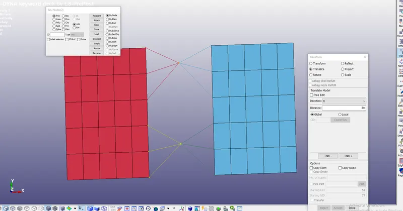
Now we have to merge the nodes with Element Tool-Trasnform-Trasnlate option and selecting the proper nodes to become coincident as shown in the image below:

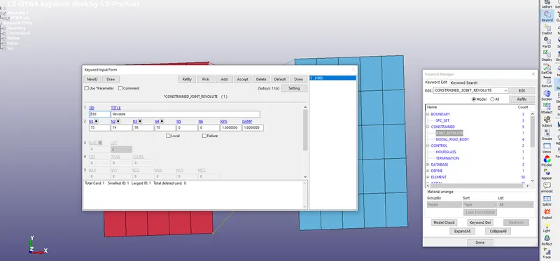
Now apply the revolute Joint under Constrained as shown in the image below like doen in case1:

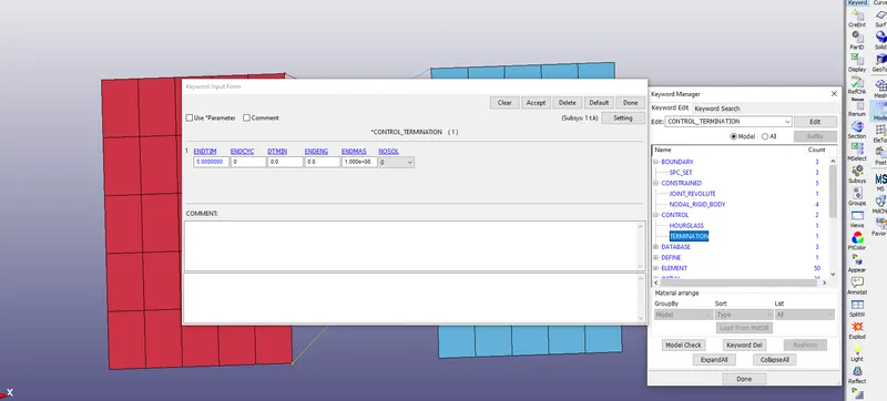
Now apply termination time with END time as 5 ms as shown in the image below:

Output Requests:

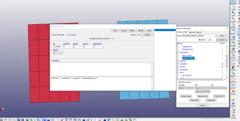
Apply Binary d3Plot under Database with DT as 0.01 ms as shown below:

Results:

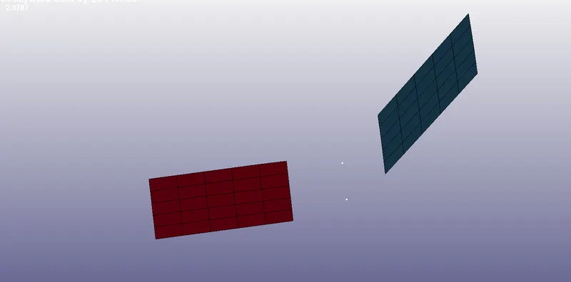
BINARY d3plot:

Spherical Joints:

Rigid bodies:

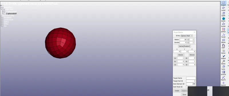
Create a speherical shell under Shape mesher option with appropriate radius as shown in the image below under meshing option:

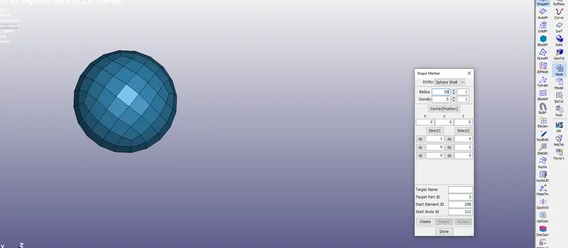
Create another Spherical shell with 50 mm radius with same centre point as shown in the image below:

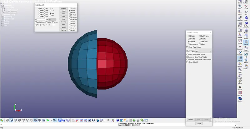
Now go to Element edit under Element tool and delete the elements of bigger sphere by hiding the smaller sphere as shown in the image:

Now create a Centre Node for both outer an Inner sphere with Element Tools-Node edit-Two nodes option for proper 2 centre node creation of 2 spheres so that one out of 2 can rotate about that centre point as shown in the image below:

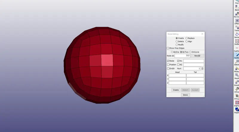
Do it same for bigger sphere as well:

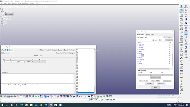
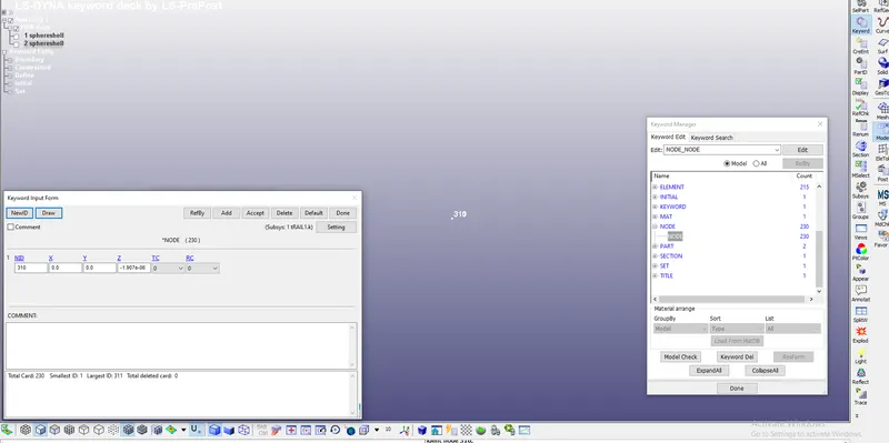
Apply the section,material and Parts same as in revolute joint with rigid bodies same material.

Boundary canditions:

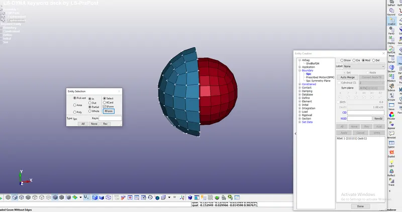
Now apply boundary canditions as SPC to fix the bigger sphere as shown in the image below:

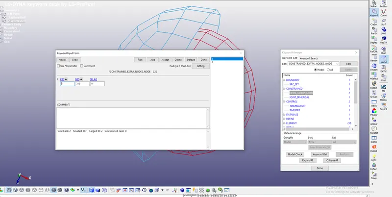
Now apply the extra node set under Constrained for rigid bodies like doen in revoulte joint as shown in the image below by selecting both the Centre nodes and 2 part IDs :

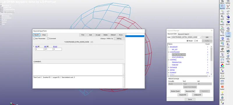
Now select the Joint_Spherical under Constrained with centre node IDs as shown in the image below:

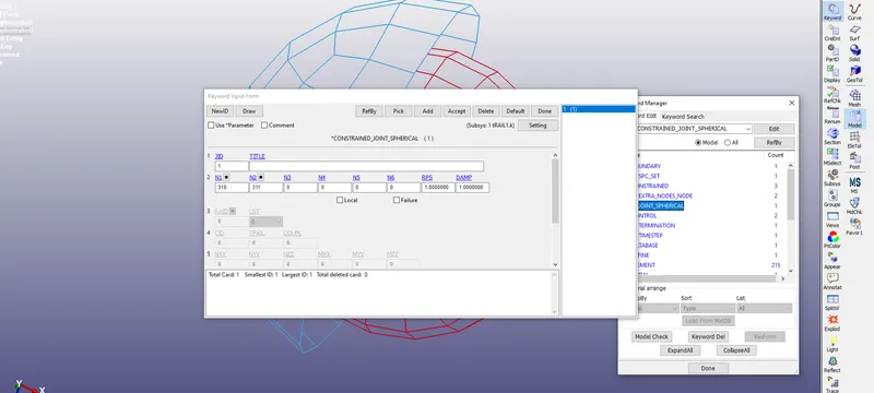
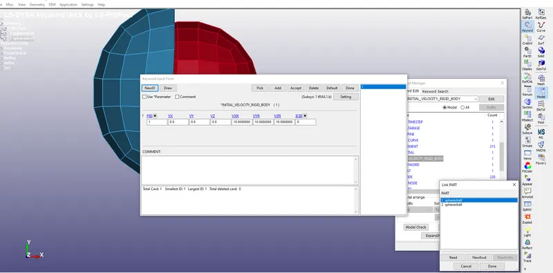
Apply Intial Velocity to the smaller sphere by selecting all its nodes and apply roatational velocity along x,y & z axis as shown in the image below:

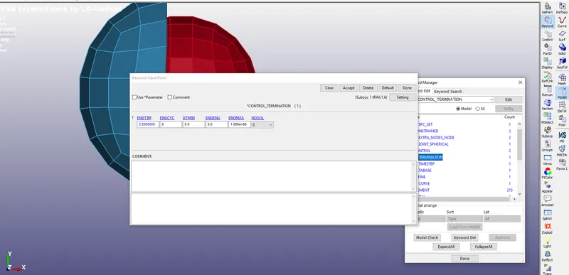
Now apply control termination with End Time as 2ms shown in the image below:

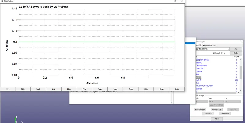
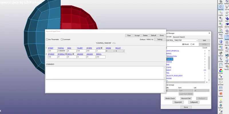
Apply Timestep as in case of Revolute joint with same LCTM under Define curve option:

Now apply Output request of Binary D3Plot under Databse with output request time DT as 0.01 ms.

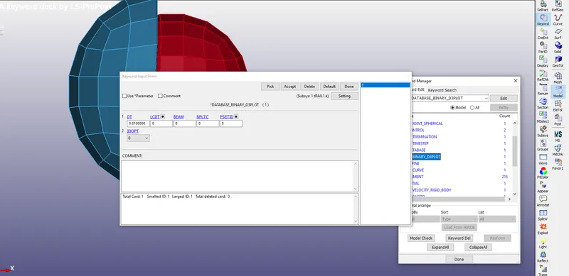
Save the model and try running it like in revolute Joint.

Results:

Binary D3PLOT:

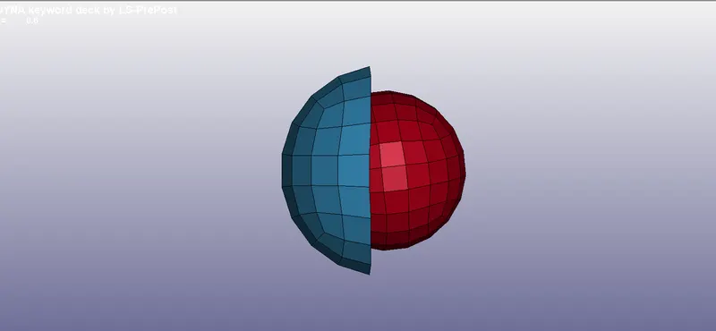
Sphereical Joint fordeformable bodies:

Change the Mat-001 Elastic as shown in revolute joint with deformable bodies.

All steps are same as in rigid bodies but in Constrained Nodal rigid body is applied by selecting outer surface nodes for both inner and outer spheres as shown in the image below:

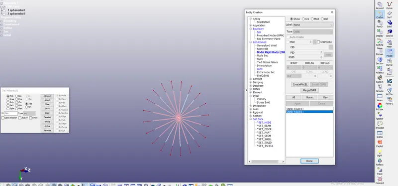
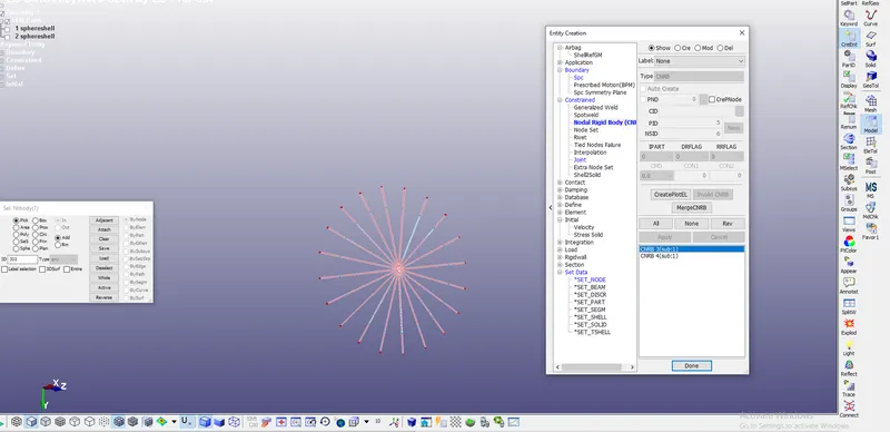
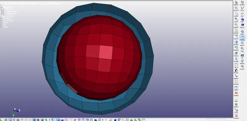
Now apply Intial Velocity to the smaller sphere by creating it sets and assigning to it as shown in the image below:

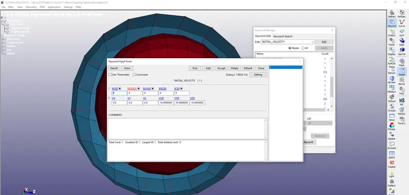
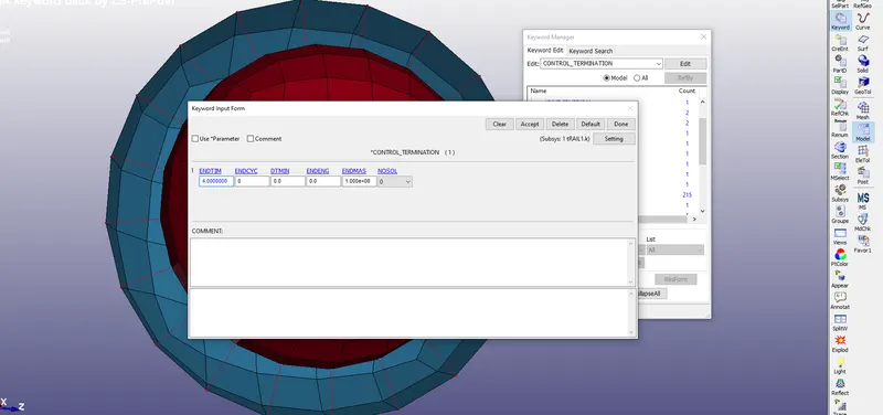
Now apply control Termination with End Time as 4ms as shown in the image below:

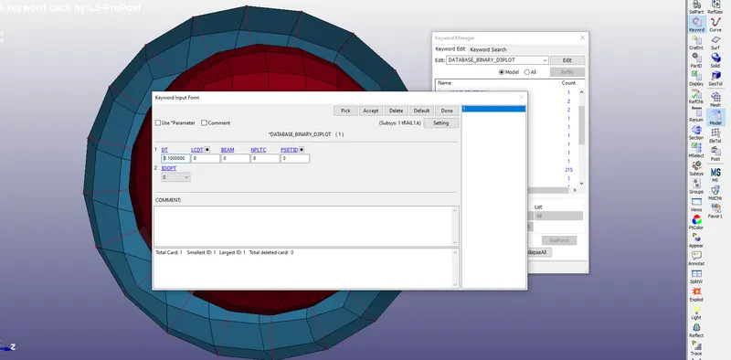
Now apply for Output requests with Database-Binary d3plot with DT as shown in the image below:

Now save the model and run the Ls dyna file.

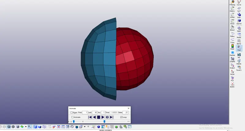
Results:

Binary D3plot:

Cylindrical Joint:

Rigid body:

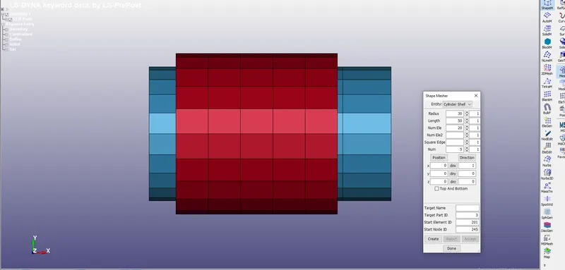
Go to the shape mesher option and draw cylindrical shell with appropriate radius and centre points & lengths as shown in the image below the final model appears:

Now create nodes by Element tools-Node edit-two point option with node ids at same points and other two different coordinates:

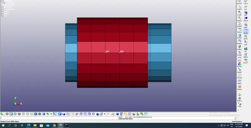
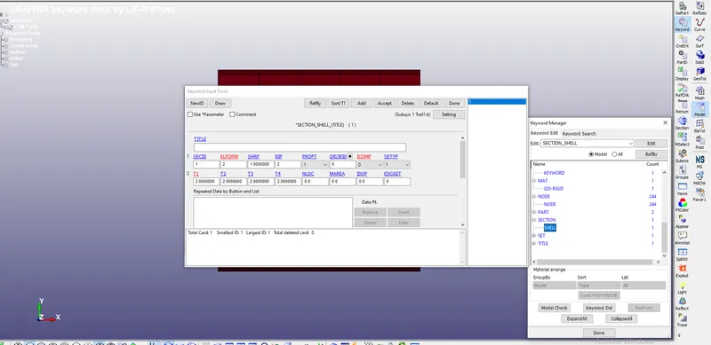
Now go to Sections under model option and select as section-shells with appropriate element formulation and thickness like that doen in prevoius two joints:

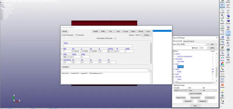
Select the materials under MAT_0020 Rigid_Body card with appropriate parameters as shown in the link below:

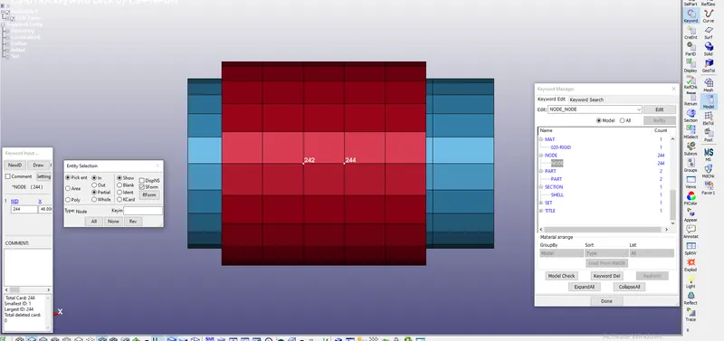
Now assign material & section to the parts:

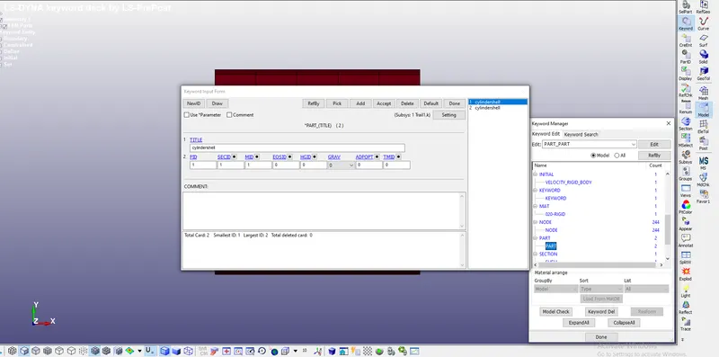
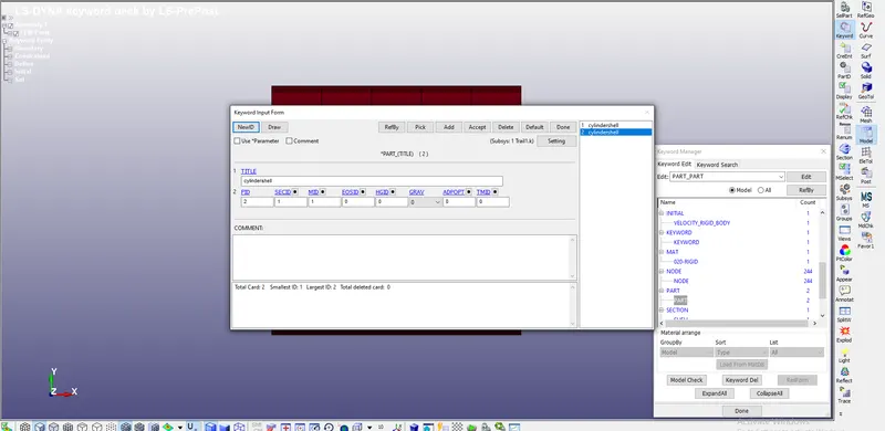
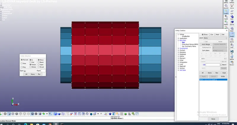
Now apply Boundary Spc to the outer cylinder by selecting all of its nodes in order to fix it as shown in the image below:

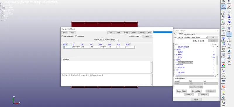
Apply Intial velocity to the inner cylinder by Inrial_Velocity rigid node option as shown in the image below along Rotational and Transverse direction with appropriate part ID:

Now apply Extra Nodes under Constrained option by selecting the the 4 centre nodes which we created for cylindrical joints by selecting any of 2 cylinders:

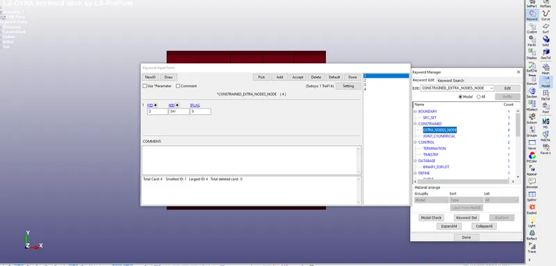
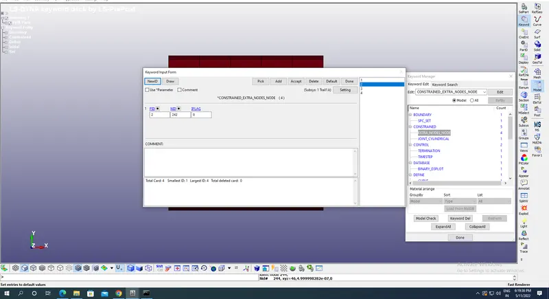
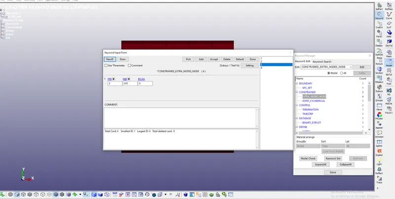
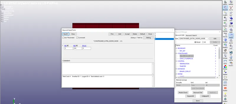
Now apply Joint cylindrical under Constrained keyword option with appropriate node id selection as shown in the image below:

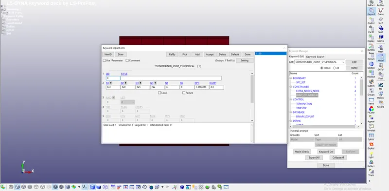
Now apply the control termination with End Time as 1.2 ms as shown in the image below:

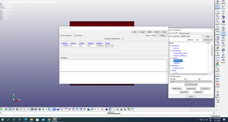
Now apply Timestep with LCTM for structural time size as shown in the image below:

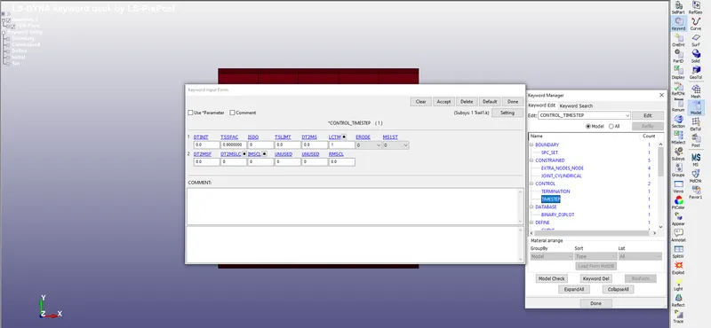
Timestep curve:

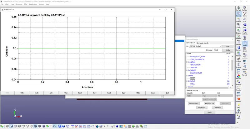
Now apply outputrequest under Database option with Binary d3plot as shown in the image below:

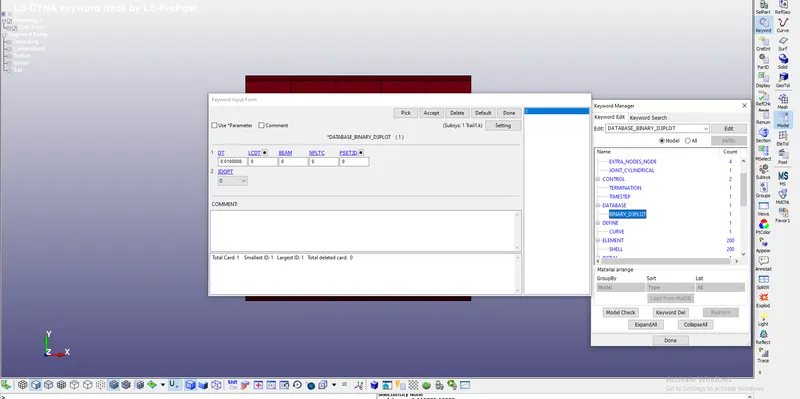
Save the model and run it for outputs.

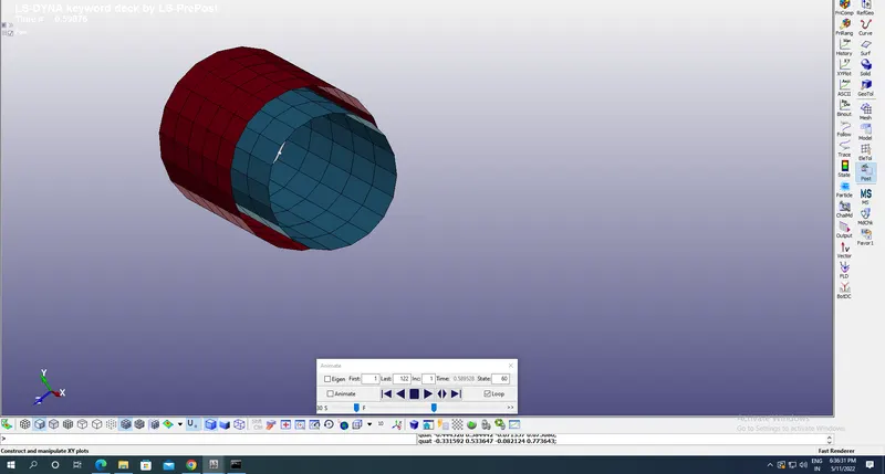
Results:

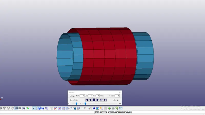
Deformable bodies:

All other setting are same as rigid only Mat card is changed to 001 Elastic as shown below:

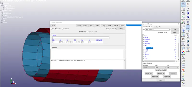
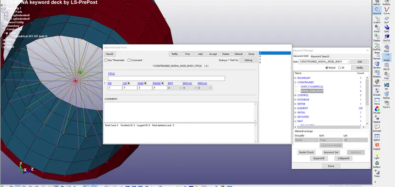
Under Constrained option instrad of extra nodes,4 Nodal Constrained rigid bodies are defined by selecting the proper nodes as shown in the image below for both the cylinder at same centres at 2 different points:

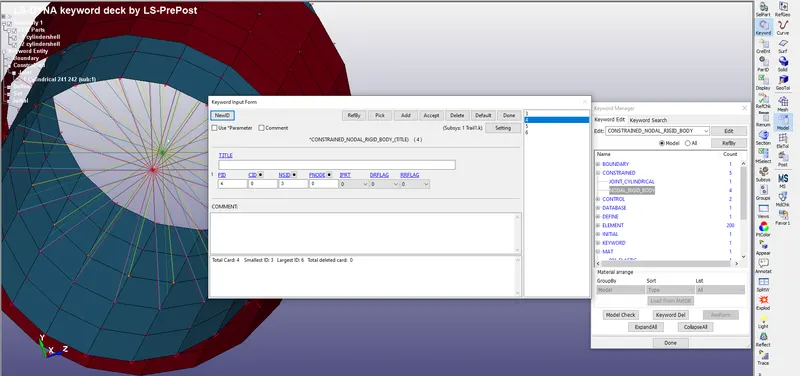
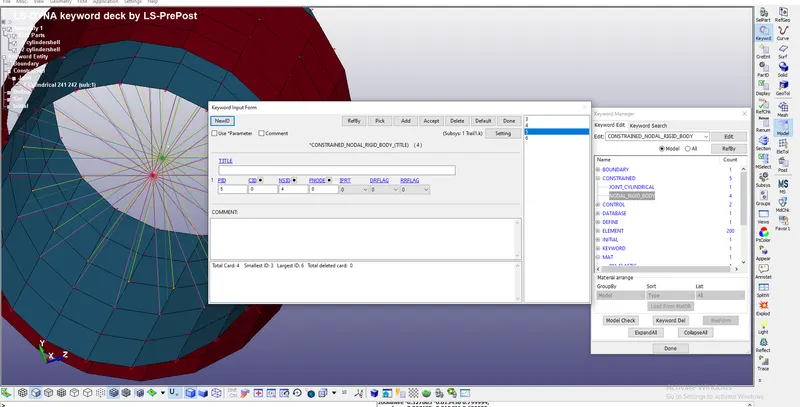
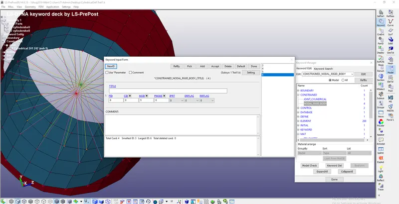
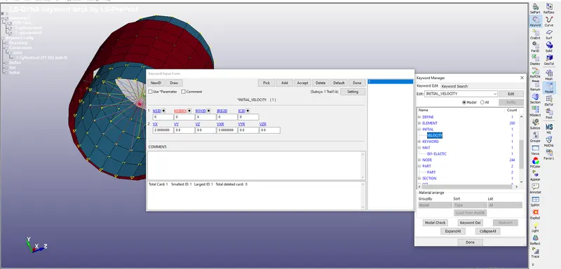
A set is created and instead of Intial rigid body like we didi for rigid here we apply the Intial-Velocity as shown in the image below:

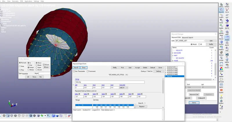
Intial-Velocity:

Results:

Binary d3plots:

Translational Joints:

Rigid bodies:

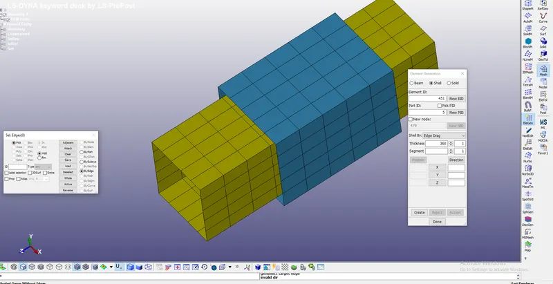
Create a 4 noded shell element by shape mesher under mesh and apply Element generation Tool and select shell by Edge Drag option as shon in the image below for both the cuboids as shown in the image below:

Assign the same section,materials by their creation,controls into the parts as doen before.

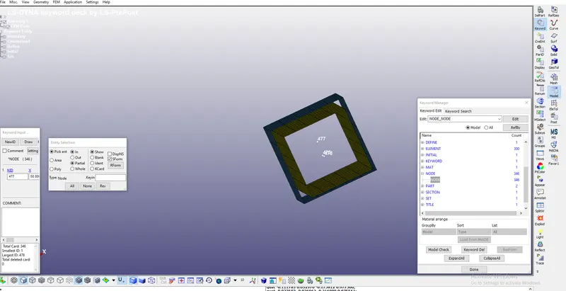
Create the 6 Nodes with middle two nodes below centreline while other 4 at centre line as shown in the image below by Elements node edit option-Two nodes:

Under Constrained define Joint TRanslational with proper centre nodes selections:

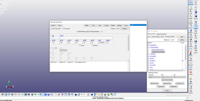
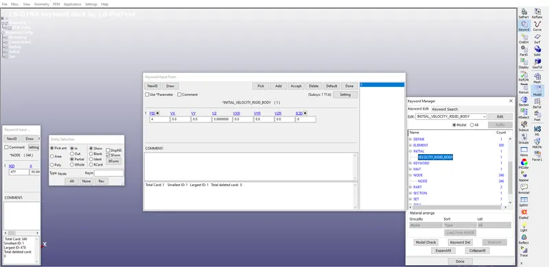
Keep all the Intial Velocity rigid body as doen prevoiusly for rigid bodies with translational velocity along Z axis to the inner cuboid as shown :

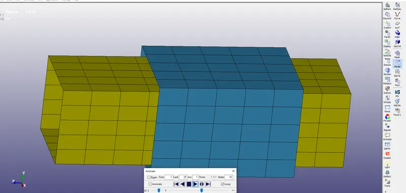
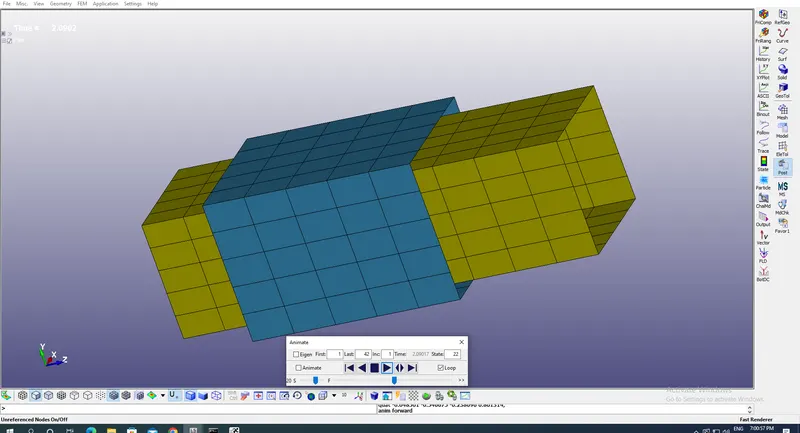
Results:

Deformable bodies:

Select the 001 Elastic material under material tab as doen for deformable body joints before:

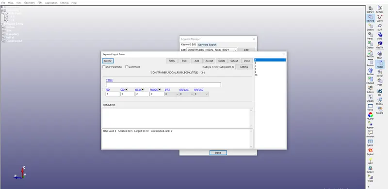
Define 6 Constrained Nodal Rigid Bodies in place of extra joints with centre nodes as shown in the image below for both the bodies:

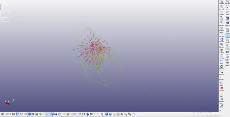
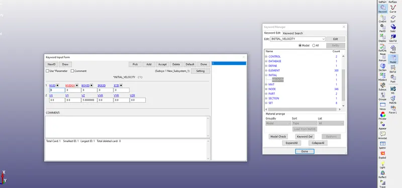
Apply Intial-Velocity of 5mm/ms under Z axis fo Deformable bodies as shown in the image below:

Results:

Binary D3 PLOT:

Conclusions:

Joints for rigid deformable bodies created and D3Plot were captured with nodes being used at centre of two bodies to create the joints like shown above.