Week-11 Challenge: Braking

Week11 Prabhu workout :

Question1

1. For a defined driving cycle, calculate the energy required for braking.

A driving cycle commonly represents a set of vehicle speed points versus time. It is used to assess the fuel consumption and pollutant emissions of a vehicle. For this challenge, the data is made as a self-defined drive cycle ‘Drivecycle_week11.xlsx’’ is considered to calculate the braking energy required.

A driving cycle commonly represents a set of vehicle speed points versus time. It is used to assess fuel consumption and pollutant emissions of a vehicle. For this challenge, the self-defined drive cycle ‘Drivecycle_week11.xlsx’ is considered to calculate the braking energy required. Prior to the start, let’s see the calculation involved to estimate the brake energy.

1 0

2 5

3 10

4 12

5 15

6 20

7 25

8 20

9 14

10 10

11 15

12 25

13 35

14 40

15 45

16 55

17 60

18 55

19 40

20 30

21 25

22 15

23 10

24 5

25 0

The process of controlling the velocity of an object by inhibiting its motion is called Braking. To bring the object in motion to a stop the kinetic energy must be removed, by dissipating the energy to the atmosphere through friction. The most common type of braking is a mechanical brake which inhibits motion through friction brake pads. Braking systems that don’t use friction are referred to as regenerative braking systems in which the kinetic energy is converted into other forms of useful energy, which can be stored for later use, increasing fuel efficiency.

As mentioned to brake the motion of the vehicle the kinetic energy has to be cut off. This Kinetic energy (Ekinetic) is given by formulating mass (m) and velocity (v) as in (eq-1)

E(kinetic) = 0.5*m*v^2 …………………………….. (eq-1)

From (eq-1) we are clear that to make Ekinetic = 0, velocity should be made ‘Zero’, Obviously m cannot be ‘Zero’. To calculate the energy the self-defined drive cycle is prepared in Excel (time v/s speed data).

Data selected -- to calculate the brake energy.

• Mass of the vehicle = Light Commercial Vehicle = Total mass = 5000kg
• Time and velocity values from the defined ‘xlsx ’

Logic adopted:

Step-1: For decelerating initial velocity Vi > final velocity V(i+1), if condition shall be used and if the condition satisfies, braking energy shall be calculated using (eq-1).

Step-2: Braking energy shall be calculated for the entire length of the drive cycle. Followed by summation and the average braking energy shall be calculated

Step-3: Braking energy shall be plotted by running the code

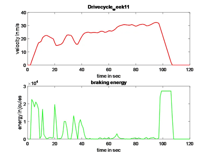
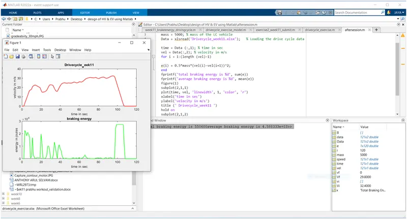
From the graph, it is evident that during the decelerating phase, the braking phenomenon takes place and the total braking energy and average braking energy required during the drive cycle are mentioned above

-------------------------------------**---------------------------**----------------------**------------

Question 2; Why electric motor can’t develop braking torque at high speed similar to starting? How electric and mechanical brakes are coordinated?

1. As we know speed and torque are inversely proportional when the vehicle runs at high speed the motor shall be operating at the constant power region during which the torque of the motor reduces which makes the motor not capable to develop the braking torque similar to the torque seen at low speeds, this is evident from the below-given torque v/s speed curve.

Observations from the above graph: At low speed, motor torque remains high, reduces as speed increases, and concludes that an electric motor cannot generate necessary braking torque at high speed similar to the one produced at initial/low speed (Hence torque is inversely proportional to speed).

b. Coordination of Electric and Mechanical braking

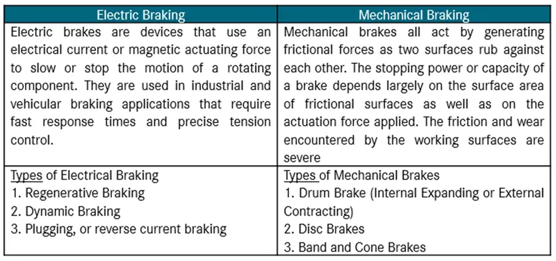
In the above table the operational method and the types of braking w.r.t electrical and mechanical are seen. The next step would be to see the control / coordination strategy that shall be used to distribute the braking activity between electric and mechanical brakes.

Two primary control techniques are Series and Parallel control strategies. Of the two methods, parallel and series (or sequential), parallel is the easiest to control as everything is somewhat linear. Pedal pressure increases both mechanical and electrical braking forces. Series systems must hold off the mechanical braking until the regenerative braking mechanism has done all it can.

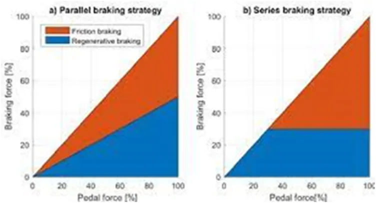
Series Control Strategy: In the first method used in vehicles with electric and hybrid drive systems to substitute the frictional braking with the electric braking, a free pedal displacement is added to the pedal travel. In such a system, a brake pedal position sensor must be used and a part of the pedal movement is made without operating the brake master cylinder. Thus, regenerative braking may be forced at small pedal displacements. At bigger pedal displacements, the driver begins to operate the brake master cylinder and the parallel braking of the vehicle is started.

Parallel braking control Strategy: The parallel braking is the simplest way to put energy recuperation into practice. The strategy of this type has been in use in the vehicles with electric and hybrid drive systems where the braking force cannot be limited automatically. For the regenerative braking to be possible, the brake pedal must be provided with a position sensor. When the brake pedal is depressed by the driver, the conventional service brake system is operated and a signal is simultaneously sent from the pedal position sensor to the converter that controls the operation of the electric machine. Usually, the converters have a separate analog or digital input through which the braking torque is set.

In recent models of hybrid vehicles like the Toyota camry : the braking force is provided with the help of an ECU-controlled motor and ball screw arrangement. This means that no direct load on the engine while applying brakes. This means that a motor operated the brake for providing the braking energy. A more controlled and uniform braking force is applied since its ECU is controlled, this helps to recover braking losses when a regenerative braking system is used. Because of its simple structure, in which the motor directly operates the brake cylinders, this new Electric Driven Intelligent Brake system has the potential to be applied to various future hybrid vehicles

Question-3

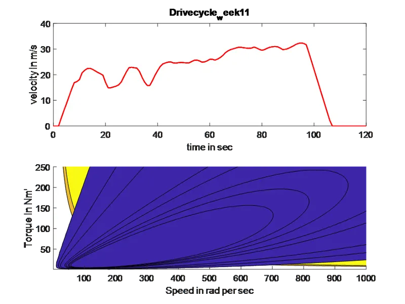
To write a MATLAB program that plots the contour of given motor speed, torque and efficiency values. The motor and the efficiency values are referred to from week 11 video-54. Code written as .m file, followed by simulation run, results observation, and conclusions. Note: .m file attached for your ref

x = linspace (1, 1000); % speed , N. B rad/s not rpm

y = linspace (1, 250); % 0 to 40 N.m

% allocate motor loss constants

Kc = 0.2; % copper losses

Ki = 0.008; % iron losses

Kw = 0.00001; % windage losses

ConL = 20; % for constant motor losses

% now make mesh

[X, Y] = meshgrid (x, y);

Outputpower = (X.* Y); % torque x speed = power

B = (Y.^2) * Kc; % copper losse

C = X*Ki; % iron losses

D = (X.^3) * Kw; % windage losses

Inputpower = Outputpower + B + C + D + ConL;

Z = Outputpower./Inputpower;

% we now set the efficients for which a contour will be plotted%

V = [0.70, 0.80, 0.85, 0.9, 0.91, 0.92, 0.925, 0.93];

box off

grid off

contourf(X, Y, Z, V);

----------------------------------**---------------------------

clc

clc

x = linspace (1, 1000); % speed , N. B rad/s not rpm

y = linspace (1, 250); % 0 to 40 N.m

% allocate motor loss constants

Kc = 0.2; % copper losses

Ki = 0.008; % iron losses

Kw = 0.00001; % windage losses

ConL = 20; % for constant motor losses

% now make mesh

[X, Y] = meshgrid (x, y);

Outputpower = (X.* Y); % torque x speed = power

B = (Y.^2) * Kc; % copper losse

C = X*Ki; % iron losses

D = (X.^3) * Kw; % windage losses

Inputpower = Outputpower + B + C + D + ConL;

Z = Outputpower./Inputpower;

% we now set the efficients for which a contour will be plotted%

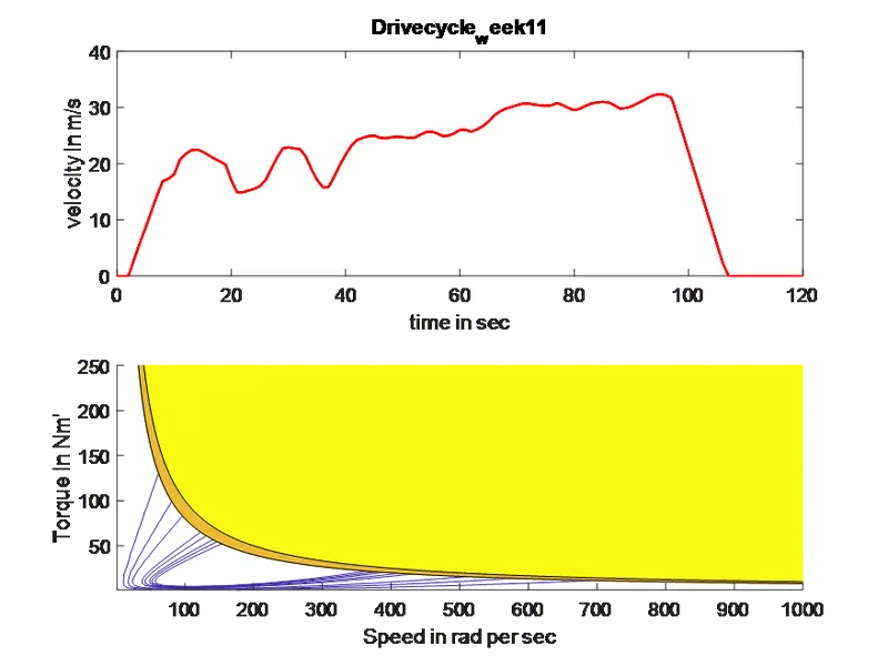
V = [8000,10000];

----------------------------------**-----------------------------------

Conclusion:

Points at innermost contour line is a set of highest efficiencies as 93%, where as points at outermost line has lowest efficiency of 70%. Which means efficiency order increases as we move inward and decreases moving outwards.

As speed increases, motor efficiency decreases.