Week-11 Challenge: Braking

Question 1: For a defined driving cycle, calculate the energy required for braking.

Answer :-

Driving cycle :-

A Driving cycle are set of vechiles speed points versus time , it is used to calculate the fuel consumption of a vechile , which is later on is compared with different vechiles. Main use of driving cycle are as follows :

• To assess the performance of a vechile (fuel economy,emissions tests)
• To analyze battery state and energy consumption in Electric vechiles
• To simulate vechile model prior to the actual development.

Braking :-

Road Vechiles involves the conversion of kinetic energy into thermal energy (heat) . when stepping on the brakes . the driver commands a stopping force several times as powerful as the force that puts the car in motion and dissipates the asscociated kinetic energy as heat.

The process of braking follows the law of conservation of energy ie. Energy cannot br created nor bre destoyrd it can be converted into another form.

E(kinetic) = 1/2*m*v^2

Matlab code for calculating Energy Required for Braking :

clear all

close all

clc

%input values

mass = 2000+0.05*(2000);

g = 9.8;

time_period = 1370;

num = xlsread('udds.xls');

time = num(1:time_period,1);

velocity = num(1:time_period,3);

decrease_in_velocity = zeros(1,time_period);

change_in_time = zeros(1,time_period);

deceleration = zeros(1,time_period);

instatenous_braking_energy = zeros(1,time_period);

for i = 1:(length(velocity)-1)

if velocity(i)> velocity(i+1)

decrease_in_velocity(i) = velocity(i+1)-velocity(i);

change_in_time (i) = time(i+1)-time(i);

deceleration(i) = decrease_in_velocity(i)/change_in_time (i) ;

instatenous_braking_energy (i) = 0.5*mass*0.001*((velocity(i))^2 - (velocity(i+1))^2)/3600;

end

end

figure

subplot(2,1,1)

plot(time,velocity)

xlabel('Time(seconds)')

ylabel('velocity(m/s)')

title ('Urban Dynomometer Driving schedule (UDDS) drive cycle data')

subplot(2,1,2)

plot(time,deceleration)

xlabel('Time(seconds)')

ylabel('deceleration(m/s^2)')

title ('Deceleration values for (UDDS) drive cycle data')

figure

plot(time,instatenous_braking_energy,'m')

xlabel('Time(seconds)')

ylabel('braking energy(kwh)')

title ('Braking energy values for UDDS drive cycle data')

fprintf('The total braking energy required for UDDS drive cycle for a time period of %d seconds is %.3f kwhn', time_period-1,sum(instatenous_braking_energy))

Results:-

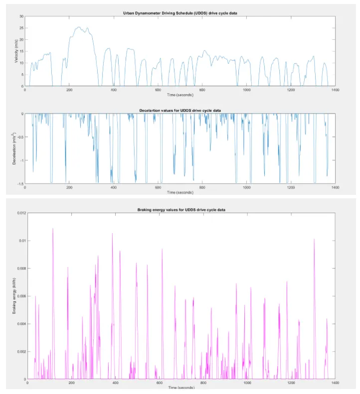
Question 2 : Why electric motor can’t develop braking torque at high speed similar to starting? How electric and mechanical brakes are coordinated?

Answer :-

An electric motor produces high torque on starting but can no genrate high braking torque while braking due to the inertia of the vechile. one way to increase braking torque is by using regenrative braking. regenrative braking in simple terms is the use of elctric motor to act as a genrator to charge the battery while slowing down or going down hill. one of the other problems with regenrative braking is that id the motor can deliver high power but the battery can not charge as fast then there is less back torque on the motor and in such cases a mechanical brake may be used.

The application of mechanical brakes along with regenrative braking can be classified into two types . they are series braking and parallel braking. in series braking the regenrative braking is used first and when we require more stopping power then the mechanical brake is used. the pattern is in series. in parallel braking the regenrative braking and mechanical brakes are used simultenously. the energy loss in parallel is more than that of series braking. as mechanical brakes convert the momentum into heat energy.

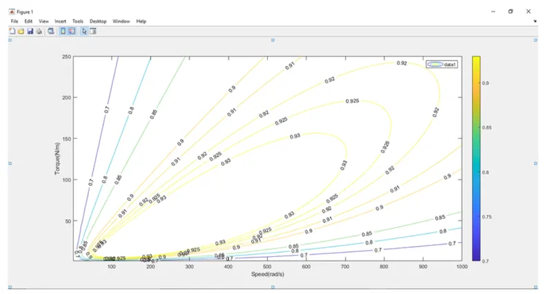
Question 3 : Make a MATLAB program which plots contour of given motor speed, torque and efficiency values. Attach the code as a .m file attach a screenshot of all the plots.

Answer :-

MATLAB CODE :-

clear all

close all

clc

x = linspace(1,1000); %speed in rad/s

y = linspace(1,250); %Torque in N/m

%motor loss constants

Kc = 0.2; %copper losses

Ki = 0.008; %iron losses

Kw = 0.00001; %winding losses

C = 20;

[X,Y] = meshgrid(x,y);

output_power = (X.*Y);

C_1 = (y.^2)*Kc ;

I_1 = (X*Ki) ;

W_1 = (X.^3)*Kw;

input_power = output_power +C_1+I_1+W_1+C;

Z = output_power./input_power

V = [0.70,0.80,0.85,0.90,0.91,0.92,0.925,0.93];

box off

grid off

[c,h]==contour(X,Y,Z,V);

xlabel('Speed(rad/s)');

ylabel('Torque(N/m)');

clabel(c,h);

Code Exlanation :-

• All the values of speed and torque are inserted using linspace command in the form of array
• A 2D grid of the arrays are created using meshgrid command.
• various motor losses and their coefficient are defined and stored.
• motor losses are calculated : copper losses, iron losses, winding losses
• input and output power calculated
• A contour is plot for the torque speed curves . efficiency is maped using clabel command.

GRAPH :-