Week-11 Challenge: Braking

Aim :

• study about the braking

Objective :

1. For a defined driving cycle, calculate the energy required for braking.
2. Why electric motor can’t develop braking torque at a high speed similar to starting? How electric and mechanical brakes are coordinated?
3. Make a MATLAB program that plots the contour of given motor speed, torque, and efficiency values. Attach the code as a .m file attach a screenshot of all the plots.

# First Objective :

Theory :

A driving cycle commonly represents a set of vehicle speed points versus time. It is used to assess fuel consumption and pollutants emissions of a vehicle in a normalized way, so that different vehicle can be compared.

we use the drive cycle of the EPA Urban Dynamometer Driving Schedule (UDDS) is commonly called the "LA4" or "the city test" and represents city driving conditions. It is used for light-duty vehicle testing.

Braking is the process of controlling the velocity of an object by inhibiting its motion. An object in motion possesses kinetic energy and to bring the object to a stop this kinetic energy must be removed

the formula of calculating the braking energy is,

Braking energy = `1/2 m(Vf ^2- Vi^2)`

Code file for calculation of braking energy :

Link:https://drive.google.com/file/d/1zLMssRcsXnAQTfYGx7zHgRlHLEK_qCy_/view?usp=sharing

clear all
close all
clc

% input mass of vehicle with 5% moment of inertia 
m1 = input('enter the mass of vehicle \n');
m = m1 +0.05*m1 ;

% time period
time_period = 1370 ;
% open the file and read the data
num = xlsread('udds_data_file.xlsx');
% extract the time data
time = num(1:time_period,1);
% extract the velocity data
velocity = num(1:time_period,2);
% decrease_in_velocity zeros(1:time_period)

decrease_in_velocity  = zeros(1,time_period);
change_in_time  = zeros(1,time_period);
decelration = zeros(1,time_period);
instantaneous_braking_energy = zeros(1,time_period);

for i = (1:length(velocity)-1)
    
    if velocity(i)>velocity(i+1)
      decrease_in_velocity(i) = velocity(i+1)- velocity(i);
      change_in_time(i) = time(i+1)-time(1) ;
      decelration(i) = decrease_in_velocity(i)/change_in_time(i) ;
      instantaneous_braking_energy(i) = 0.5*m*0.001*((velocity(i))^2-(velocity(i+1))^2)/3600 ;  
    end
    
end

fprintf('total braking energy required for UDDS drive cycleis of time %f is %f KWh',time_period , sum(instantaneous_braking_energy))

figure(1)
plot(time,velocity);
xlabel('time(sec)')
ylabel('velocity(m/s)')
title('Urban Dynamometer Driving Schedule')
grid on 

figure(2)
plot(time,decelration,'g');
xlabel('time(sec)')
ylabel('decelration(m/s^2)')
title('Urban Dynamometer Driving Schedule')
grid on 

figure(3)
plot(time,instantaneous_braking_energy,'r');
xlabel('time(sec)')
ylabel('braking energy (Kwh)')
title('Urban Dynamometer Driving Schedule')
grid on 

In the above file, we input the mass of the vehicle as 2000 with an approximate 5 % moment of inertia

Then we declare the time period 1370 sec from the drive data.

using the xlsread function we open and read the file data. we declared with the variable as num.

From that, we extracted the time and velocity data and store it as variable time, velocity respectively.

decrease in velocity, change in time, deceleration, instantaneous braking energy is initiated as zero using the function zeros for all up to the time value.

Then in the for loop, we check for the condition that if the velocity(i) is greater than velocity(i+1) the for that value we calculated the instantaneous braking value and deceleration value and end the loop

then we printed the sum of all instantaneous values of braking energy.

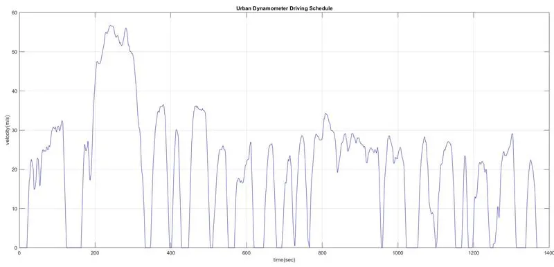
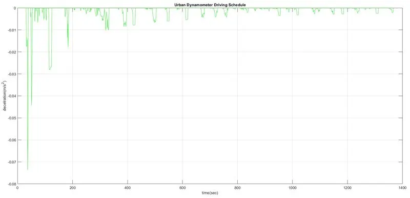
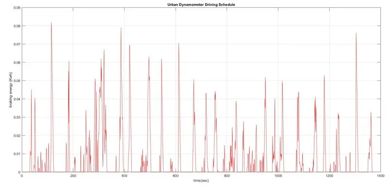
Then we plotted the time velocity, time deceleration, time braking energy graph for the UDDS drive cycle.

Braking total energy in (kWh)

for the 1370 sec drive cycle of 2000 kg weight vehicle uses the around 6 kWh of the braking energy

the plot from the UDDS data :

plot for deceleration :

Braking energy plot :

# Second Objective :

Why electric motor can’t develop braking torque at a high speed similar to starting?

Below we have shown the speed-torque characteristics of motor

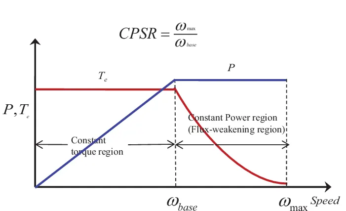
Here it cleared that in the torque-speed curve that till we reach the critical or base speed it has constant torque and once it reaches the critical speed the curve has a downslope which is the constant power region which shows the accelerating operation of the motor. For the decelerating operation motor, this graph is mirrored down which will be having a positive speed and negative torque

for example :

we can say that EV can achieve 0-100 in 10 sec. Acceleration operation goes this way, with low speed and high torque constant torque region is achieved which has accelerating power and by reaching the critical speed it shifts to constant power region and thus it is for EV to reach 0-100 kmph

as we said the braking operation is mirror images of the above plot so we can not say that the motor producing some positive torque for acceleration can also produce some negative torque for braking. Because we operate in the field of weakening region and operating and above the base speed. Thus peak acceleration torque will be greater than peak deceleration torque. Thus for acceleration, it has a high torque with the low speed and for deceleration, it has low torque high speed

Mechanical and electric braking system coordination :

Generally, there are two types, first is regenerative and mechanical brakes. the brake force is distributed in both regenerative and mechanical braking systems.

what is the regenerative braking

Regenerative braking turns your car's kinetic energy into electricity to charge its battery and boost efficiency. The resulting friction works to slow the car down, generating heat and wearing away at the material on the pads and discs in the process.

what is mechanical braking?

Brakes absorb energy and convert it to heat. Mechanical brakes all act by generating frictional forces as two surfaces rub against each other. The stopping power or capacity of a brake depends largely on the surface area of frictional surfaces as well as on the actuation force applied.

mechanical brakes use the drum of disc mechanism for applying the brakes.

The brakes are further divided on the basics of the brake control strategies:-

• series
• parallel

In series braking the brakes are applied one after the other may be like regenerative first and mechanical or vice versa. they are applied one at a time we can use such types of braking control strategies where we can require comfortable and efficient braking

In the parallel strategies both the brakes are applied at a time

as per the system developed by the Nissan leaf electric driven intelligent brake (EDIB)coordination of the brake system is been plotted

Brakes absorb energy and convert it to heat. Mechanical brakes all act by generating frictional forces as two surfaces rub against each other. ... The stopping power or capacity of a brake depends largely on the surface area of frictional surfaces as well as on the actuation force applied.

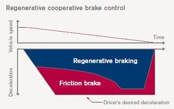
as from the graph, it is clear that high the speed of vehicle percentage of frictional brake or mechanical brakes are applied is higher as compared to regenerative brakes but as the speed of the vehicle is decreasing the percentage of brake ratio is changing and the regenerative brake are applied in greater ratio as compared to mechanical brakes.

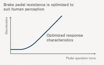
in the above graph of brake pedal resistance, we can see that as the brake operation force is increased the rate of deceleration is also increased. The percentage of the ratio of regenerative and friction braking is decided by the position of the brake pedal

# Third Objective :

• to plot the contour line of the motor.

Copper Losses - `I^2*R`, Where R is armature resistance and we say Torque is proportional to current, this copper loss can be considered as. where is to take care of resistance of brushes and also take care of ux and its effects.

copper losses = `Kc*T^2`

Iron losses - Iron losses are nothing but magnetic losses, which is denoted as, where the factor is based on the magnetic eld effect. for permanent magnets have constant magnetic eld and iron losses is based on the value and this is going to change according to the speed.at various speeds have a different value of back EMF and that is going to affect the iron losses.

iron losses =`Ki*omega`

Windage losses - This is a mechanical or friction of windage losses this is based on the size of the motor and the number of windage losses that the motor is going to experience.

Constant losses -

this denoted as C

Total losses are considering the above four losses and denoted as,

Total losses = `Kc*T^2 + Ki*omega +Komega *omega^3 +C`

All the motors are model as per the above equation of losses. This above equation is not only applicable for permanent magnet DC motor but other as well like induction motor

Matlab program :

link for code:https://drive.google.com/file/d/1dgSWsE9znHfiw36VcoevZM_Kjs08kM5K/view?usp=sharing

clear all 
close all
clc

% speed array 
w = linspace(0,1000) ;
% Torque array 
T = linspace(0,200) ;

% losses coefficients
kc = 0.18;       %copper losses
ki =0.006;       % iron losses
kw = 0.00015;    % windage losses 
  
% meshgrid  
[x,y] = meshgrid(w,T);
copper_loss = (y.^2)*kc ;
iron_loss = x*ki ;
windage_loss = (x.^3)*kw ;
constant = 20 ;

o_p = x.*y ;
input_power = (copper_loss)+(iron_loss)+(windage_loss)+(o_p)+constant ;
eff = (o_p)./(input_power) ;
n = linspace(0.7,0.95,10) ;

contourf(x,y,eff,n,'linewidth',2)

box off 
grid on 
title('speed torque chracteristics')
xlabel('speed rad/sec')
ylabel('torque Nm')

We created the speed array and torque array using linspace function.

Then we input the losses coefficients as the variable Kc, Ki,Kw.

Then we use the meshgrid function as variable x and y with arguments of w and T.

with the above formula, we formulized the copper losses, iron losses windage losses, constant.

Then we calculated output using the x and y values.

Then input power is calculated by adding all the losses. efficiency is calculated by dividing the output by input.

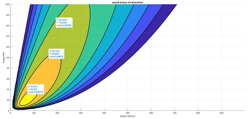
using the contourf function plot the contour of x , y, and efficiency

plot :

#Conclusion :

• In the first objective, we calculated the braking power for the UDDS cycle.
• In the second objective, we explain Why electric motors can’t develop braking torque at high speed similar to starting andHow electric and mechanical brakes are coordinated?
• In the third objective, we plotted the contour.