Week-11 Challenge: Braking

AIM:

1. For a defined driving cycle, calculate the energy required for braking.
2. Why electric motor can’t develop braking torque at high speed similar to starting? How electric and mechanical brakes are coordinated.?
3. Make a MATLAB program which plots contour of given motor speed, torque and efficiency values. Attach the code as a .m file attach a screenshot of all the plots.

ANSWERS:

1. For a defined driving cycle, calculate the energy required for braking.

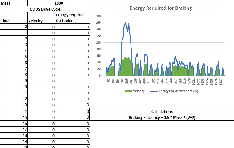
Calculating the energy required for braking of UDDS Drive Cycle-

Braking: Braking is a condition to slow down or stops a moving vehicle as required. There are several techniques to apply brakes, which can be mechanical or electrical. The most commonly used technique is by applying friction. It consumes energy .The consumed kinetic Energy can be derived as following equation-

Braking Energy = (1/2)*m*v^2

Where, Braking Energy is the kinetic energy in unit of Joule.

m= Total Mass of the Vehicle (Vehicle Mass + Pay Load) in unit of Kg.

v= (Initial Velocity-final Velocity) in unit m/s.

For Example if Initial speed of a vehicle is 20m/s and final speed is 10m/s. The mass of the vehicle is 500kg. Then the required kinetic energy for Braking is (1/2)*500*(20-10)^2 = 25000 J =25KJ

Here for a Drive cycle the required braking energy is calculated for each second of time to slow down or stop the vehicle- Braking Energy Calculation for UDDS Driving Cycle

2. Why electric motor can’t develop braking torque at high speed similar to starting? How electric and mechanical brakes are coordinated?

• Why electric motor can’t develop braking torque at high speed similar to starting?

When the motor is at rest and it has to operate from standstill position to the reach the moderate speed the higher torque is required to bring the motor in operation. Whereas when the vehicle is already at high speed the capping or the limit is reached by the motor operation and thus any further higher torque could not be obtained while braking. The braking operation happens in the motion which is been distributed as per proportion in the BRAKE ENERGY and the REGENERATIVE BRAKING.

• How electric and mechanical brakes are coordinated?

In Mechanical braking which we usually see and experience in all vehicles the brake pedal in the vehicle cabin helps us to engage or disengage the brakes. Currently the braking technology have done wonders by inventing life saving braking technologies such as ABS, EBD, BA and mny others. All these technologies play vital role in stopping the vehicle and coming back to rest from a high speed. In all these vehicles when the driver applies the brakes the brake peds come closer to the disc connected with the driving disc. The brake pads usually help in efficient braking.

There are two generic methods by which the vehicle could be braked in the ELECTRIC BRAKES.

Series - The Regenerative Braking or the Mechanical Braking noth are applied one after another.

Parallel - The Regenerative Braking or the Mechnical Braking both are applied Parallely.

When the brake pedal is pressed the hydraulic fluid reaches the brake piston and created the braking pressure on the wheels and the same kinetic energy is been used by the Regenerative Braking for generating more power using the Bi-directional motor which operates as a generator while braking.

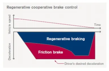
An example of the proposition of Regenerative Braking and the Mechanical Braking

NISSAN LEAD - EDIB (ELECTRONIC DRIVEN INTELLEGENT BRAKING)

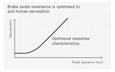
EDIB (Electric Driven Intelligent Brake) controls the regenerative brake and friction brake to support both of these requirements. Further, it also controls the reactive force from the pedal in order to unify the feeling when stepping down on the pedal and the sense of deceleration.

3. Make a MATLAB program which plots contour of given motor speed, torque and efficiency values. Attach the code as a .m file attach a screenshot of all the plots

MATLAB Code:

.m file link

https://drive.google.com/file/d/1sCENjdXLXQ3UEmnXoXMF_dgcRYt06nx6/view?usp=sharing

clear all
close all
clc
%speed  array
w = linspace(0,300,100);

%torque array
T = linspace(0,2000,100);

%meshgrid
[X,Y] = meshgrid(T, w);

%loss coefficients
cu = 0.17;              %copper coefficient
fe = 0.006;             %iron coefficients
win = 0.000015;         %windage coefficients

%losses
cu_loss = cu*(Y.^2);    %copper loss
fe_loss = fe*(X.^2);    %iron loss
win_loss = win*(X.^3);  %windage loss
cond_loss = 18;         %conduction loss

%output power
P_out = (X.*Y);
%input power
P_in = P_out + (cu_loss) + (fe_loss) + (win_loss) + (cond_loss);
%Efficiency
n = ((P_out)./(P_in));

%Efficiency values for contour
W = linspace(0.75, 0.95, 10);

%contour plot
contour(X,Y,n,W)
xlabel('Angular speedd,rad/s')
ylabel('Torque,Nm')
title('speed,torque and efficiency characteristics of motor')

Explanation:

In this MATLAB script, we create arrays for the speed and the torque of the motor using the ‘linspace’ command. For the speed, consider a range of values from 0 to 2000 radians per second whereas for the torque, consider a range of values from 0 to 300Nm.These arrays are then used to create 2D grid coordinates using the ‘meshgrid’ command. These coordinates will help in the creation of the contour plot. In order to find the efficiency of the motor, we need to consider the various losses that occur in the motor’s operation. These are:

Copper losses

Iron losses

Windage losses

Conduction losses

These various losses are dependent on the speed and the torque of the motor. They each also have a characteristic constant of proportionality which are all assumed for the following calculations and represented as 'K'. In each calculation, the speed and the torque are represented respectively as: ω and T.

Copper losses = KCu⋅ω2

Iron losses =KFe⋅T2

Windage losses =Kw⋅T3

The values of coefficients are taken as general values. Conduction losses are assumed to be 18 Joules.

Finally we plot the contour with the 'contour' command. In addition, an array for the efficiency values we want to plot for is created called 'W' and is assigned for values ranging from an efficiency level of 0.75 to 0.95. This array is used in the creation of the contour. Axis labels and a title is also made for better readability.

Output:

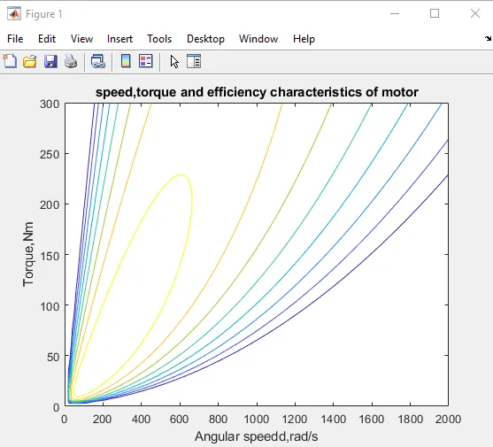
From this contour plot, we can see that the highest level of efficiency arises in the innermost contour plot and this efficiency decreases as the contours increase in size from the innermost contour.