Week 11- Broadband Noise modelling over Ahmed body
BROADBAND NOISE MODELLING OVER AHMED BODY
1 INTRODUCTION
1.1 Ahmed body
An ahmed body is a generic car body, also a simplified car model. The airflow around the ahmed body characterises the essential flow features around an automobile body. It is used for numerical validation and describing turbulent flow features. It has a rear slant portion with variable slant angle.
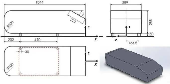
It was first used with experimental data to validate turbulent flow models. The experimental setup includes LSTM (Low Speed Wind Tunnel) and a 2-component Laser Doppler mounted on a traversing system. The flow region which contributes more to the automobile's drag and hindrances to numerical predictions is the wake flow after the slant portion of the model. The location at which the flow separates describes the flow separation and also the drag force. The significance of this model lies in validation of the exact simulated predictions.
1.2 Aero-acoustics
The generation of sound by a turbulent flow is the most common physical effect associated with the field of aeroacoustics. The prefix aero means air, however, the field of aeroacoustics is not restricted to flow-induced noise in air. Aeroacoustics is concerned with the general interaction between a background flow and an acoustics field. For example, if you were studying the reflections of sound off a shear layer or how the flow in a muffler affects transmission loss, you would be studying aeroacoustics. Aeroacoustics models can include effects that alter an acoustic field in the presence of a flow, such as turbulence, local variations in material properties, convection, viscous damping, and much more. Numerically solving aeroacoustic problems falls under the field of computational aeroacoustics (CAA).
Acoustic noise generated by a flow can be created through different mechanics, but is ultimately due to fluctuations in the flow. These fluctuations will give rise to distributed acoustic sources throughout the flow. Noise is created by local stress fluctuations in the flow (Reynolds stresses, viscous stress effects, and nonisentropic effects all act as quadrupole sources); pressure fluctuations at walls (e.g., dipole sources at solid boundaries); mass and heat fluctuations (e.g., distributed monopole sources); and external fluctuating force fields.
Acoustic waves are only a subset of waves that are created by the flow; vorticity and thermal instability waves are also produced. These particular waves are only convected by the flow, whereas acoustic waves also propagate relative to the flow, at the local speed of sound. Compared to other fluctuations, the energy associated with acoustic waves is typically many orders of magnitude smaller. This means that a direct simulation of the flow-induced noise is very challenging and requires extremely accurate numerical schemes. Another difficulty is that the acoustic sources occur at the length scale of the turbulence in the flow, which then needs to be resolved.
Acoustic analogy equations are formulations that separate out acoustic fluctuations from flow fluctuations. The first form of these equations derived from the seminal work of J. Lighthill in the 1950s. His acoustic analogy equation is obtained by rearranging the Navier-Stokes equations, which result in a convected scalar wave equation for the acoustic pressure and a right-hand side that contains all of the flow source terms. Analogy equations can also be constructed by rearranging the flow equations in other ways, leading to linearized Euler equations or linearized Navier-Stokes equations with right-hand side flow sources. The linearized models have great applicability in many aeroacoustics situations where the flow-induced noise is not important. This is found in fluid-structure interaction (FSI) problems in the frequency domain, when modeling how a background flow affects the acoustics (e.g., reflection and refraction), detailed muffler models, and much more.
Ideally, aeroacoustic simulations would involve solving the fully compressible Navier-Stokes equations in the time domain. Acoustic pressure waves would then form a subset of the fluid solution. However, this approach is often impractical for real-world applications, due to the computational time and memory resources required. Instead, like solving for many practical engineering problems, a decoupled two-step multiphysics approach is used:
1. Solve for the fluid flow
2. Solve for the acoustic perturbations on top of the flow
Several models exist that include different levels of detail and different aeroacoustic effects. These models are derived by linearizing the dependent variables around a steady-state background flow and making physical assumptions. The dependent variables now represent perturbations, such as acoustic and instability waves, on top of the flow. The classical scalar wave equation, otherwise known as the Helmholtz equation in the frequency domain, is an example of a linearized model with no explicit losses and an isentropic assumption
2 COMPUTATION OF THE DOMAIN
2.1 Geometry and meshing
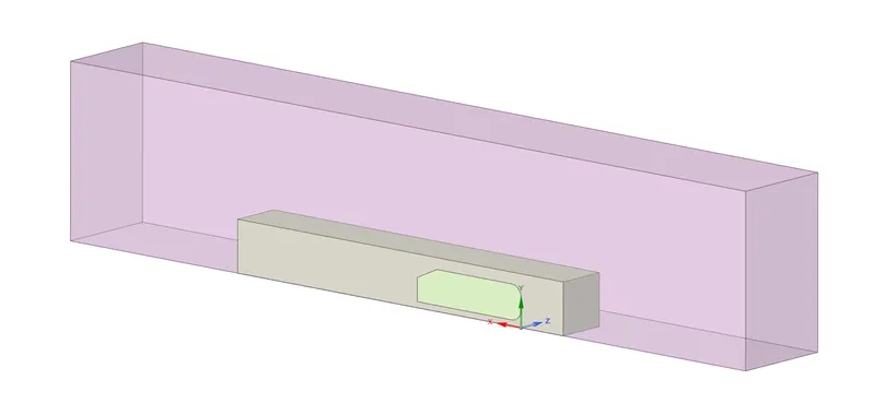
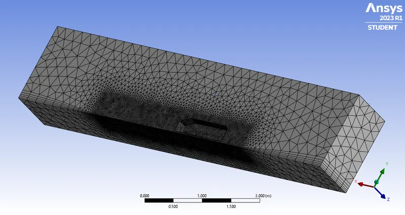
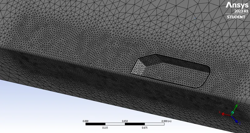
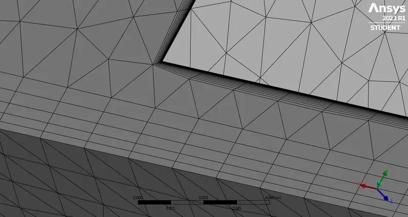
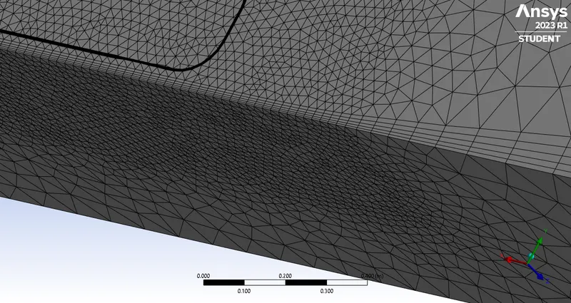
Basic element size = 200mm
Body sizing = 27 mm
Inflation of ahmed body = 28 layers with first cell height 0.01mm
Inflation of bottom face = 5 layers with smooth transition
Total number of elements = 472186
2.2 General solver settings
Model: A pressure based, steady state, K-Epsilon Realizable model with enhanced wall treatment
2.3 Material and Cell zone conditions
Air is chosen as the material and all the cell zone as designated as fluid.
2.4 Boundary conditions
The bottom face of the wind tunnel is named as the road and is set for a translational movement at 31m/s.
The inlet is a velocity inlet with 31m/s fluid velocity.
The wall and symmetry conditions are used as per the geometry.
Standard initialization is done from the inlet and the solution is controlled with a low courant number of 10.
2.4 Broadband modelling
Acoustics model is turned on and separate contours are computed for
i. Acoustics power level (dB)
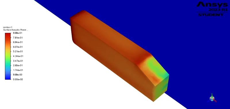
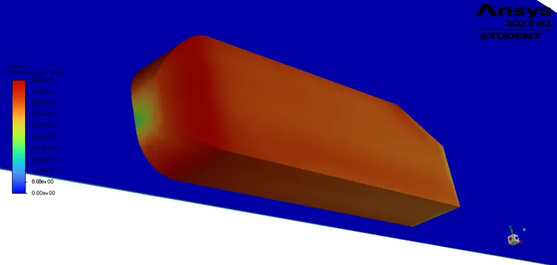
ii. Surface acoustic power level (dB)
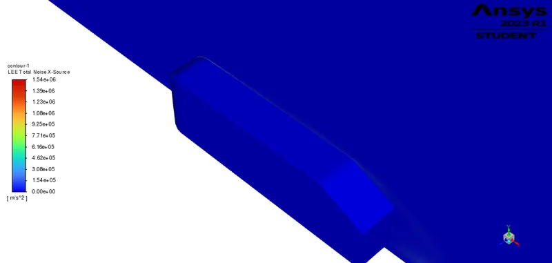
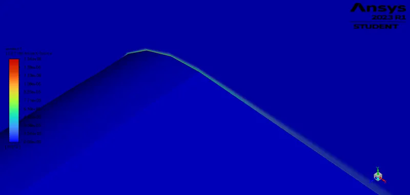
iii. Lilley's total noise source
3 RESULTS
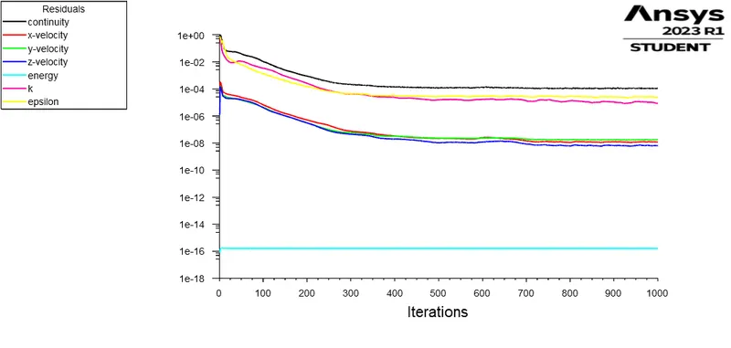
3.1 Residuals plot
3.2 Cl and Cd plot
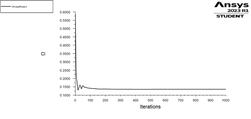
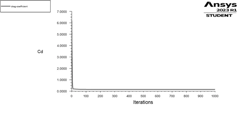
Computed Cd = 0.161 ; Computed Cl = 0.135
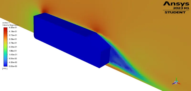
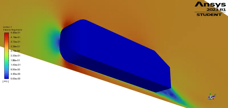
3.3 Velocity plot
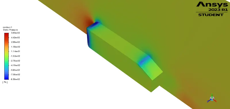
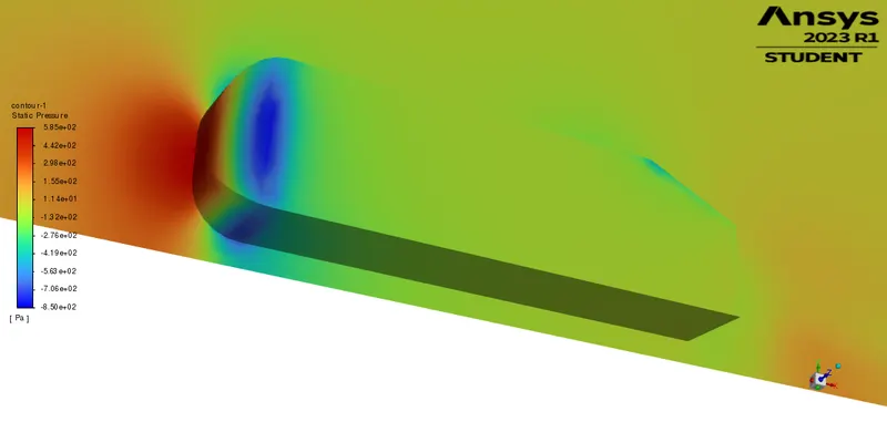
3.4 Static pressure plot
3.5 Total pressure plot
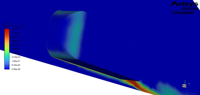
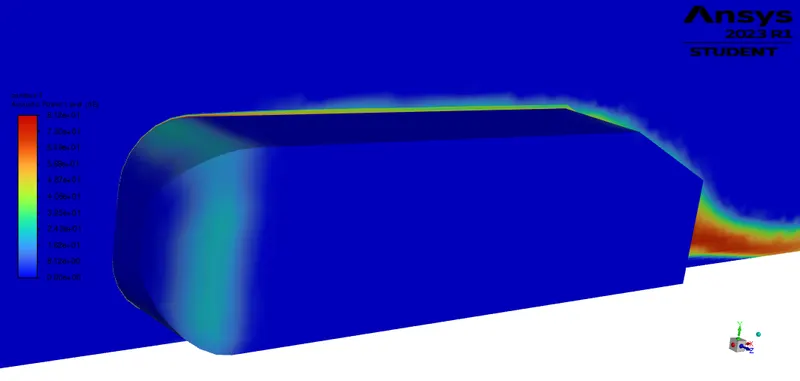
3.6 Acoustics power level (dB)
3.7 Surface acoustic power level (dB)
3.8 Lilley's total noise source
4 INFERENCE
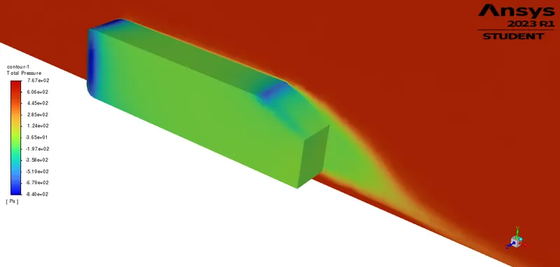
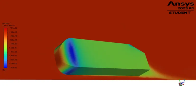
The results show that the residuals have converged pretty soon with the Cl and Cd plots also. From this it can be interpreted that the solver and the viscous model is fairly suitable for this kind of problem. The Cl is calculated as 0.135 which is an attribute of the shape of the Ahmed body and the velocity of the free stream. The Cd is 0.161 which is more than Cl as the shape of the Ahmed body has an angle front profile and a sudden slant in the rear profile which gives a loss in fluid velocity as the boundary separation occurs for such an angle and an increase in drag coefficient has been recorded. The velocity plot shows that velocity on the surface of the body is less while it is more for the particles surrounding the body in the free stream. The velocity plot also gives the rear-end trail behind the vehicle body which shows the vorticity of the fluid particles induced by the body in motion. The pressure plot tells the point of high pressure created at the tip of the frontal face of the body, due to its aerodynamic profile. The total pressure is high around the near field of the vehicle body, while it is low in the fluid field surrounding the body. The curvature in the frontal portion and the slant in the rear portion of the vehicle body is factor for the diversity in the fluid flow properties.
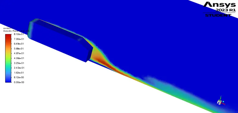
The turbulence of the fluid which causes aerodynamic noises is calculated in the aeroacoustics module of Ansys fluent. The source terms are the terms that cause the vibrations and the parts which cannot absorb these disturbances tend to emit more noise. These parts are identified and the parameters are measured in the module based on the mesh, geometry and the free stream conditions. Form Lilley total noise plot, it can be observed that the source of maximum noise is due to the particles vibration on the interface of the body and the free stream. The acoustic seems to be high at the surface of the body and is little less at the back side of the body as there is boundary separation at the back end and this reduces the vibration and noise emission. The epoch created at the backside of the body can also be observer in the plot and this is the sound that is heard by a passerby human when a vehicle passes, and this is due to the entire aerodynamic behaviour of the body.