Week 11- Broadband Noise modelling over Ahmed body

Objective:

In this challenge, you are required to do the following.

1. Describe Ahmed's body and its importance.
2. Setup the domain and setup assuming body is travelling at 110 kmph
3. Run the setup till convergence and plot for static pressure and coefficient of drag and lift to check for convergence
4. Turn on Broadband- modelling and detail the acoustic field study over Ahmed body.

Answer:

Part 1: Describe Ahmed's body and its importance.

Ahmed body is the generic car model which is used in the industry as reference or for research purposes to study different aerodynamic characteristics.

Part 2: Setup the domain and setup assuming body is travelling at 110 kmph.

The objective of the simulation is to study the acoustic field generated by the Ahmed Body.

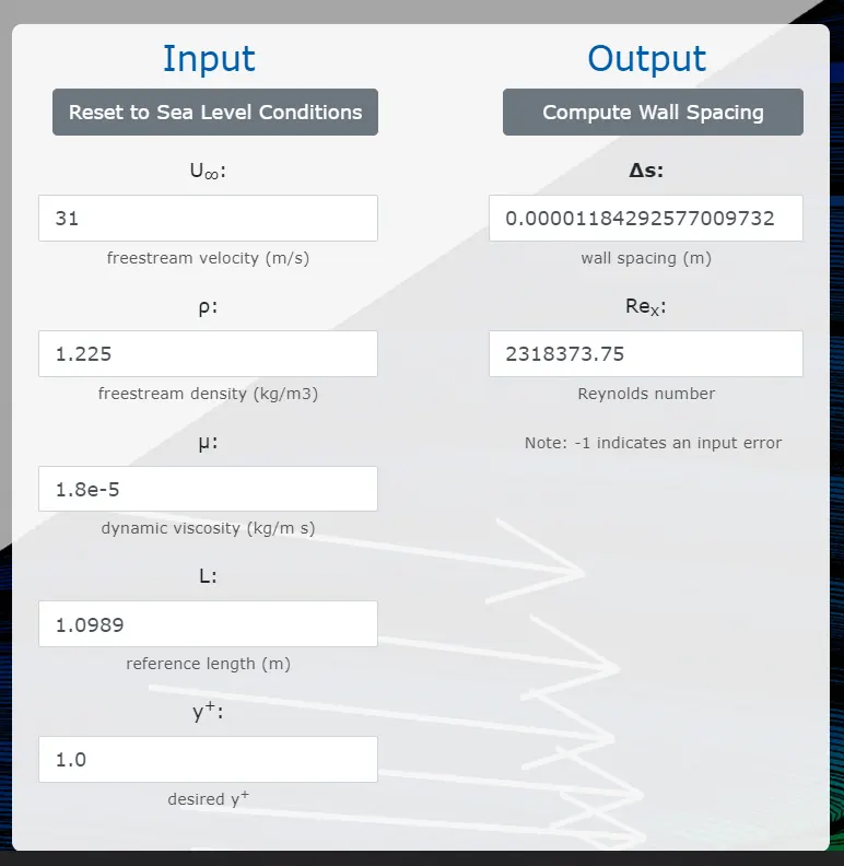
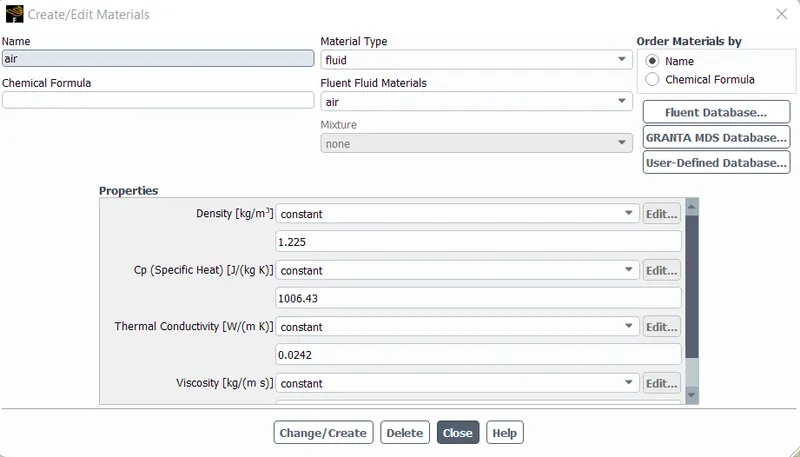
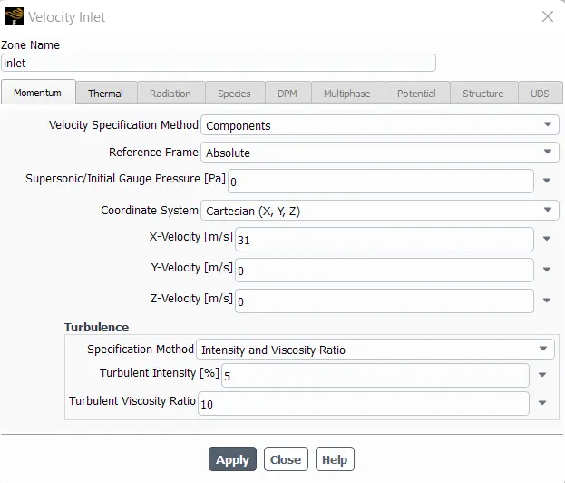
Velocity = 110 kmph = 31 m/s

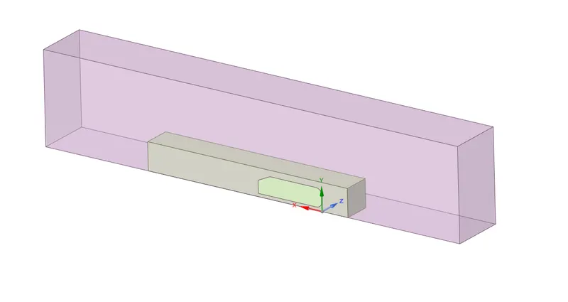
Given Model:

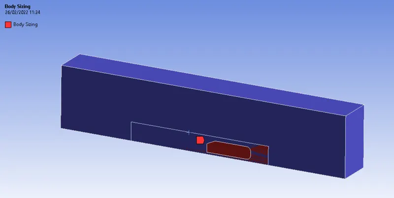
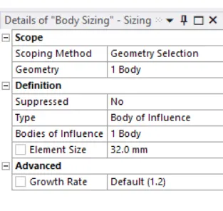
Inside smaller box is for the denser region which will be used as "body of influence" later in the Ansys Meshing.

y+ calculation using Pointwise Calculator for 1st wall thickness & Reynolds number.

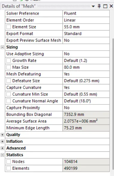
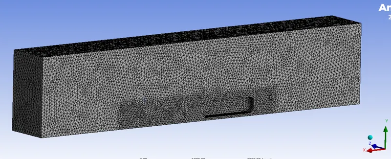
Global Mesh Settings

Denser Region

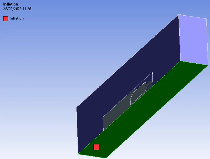
Inflation - Road

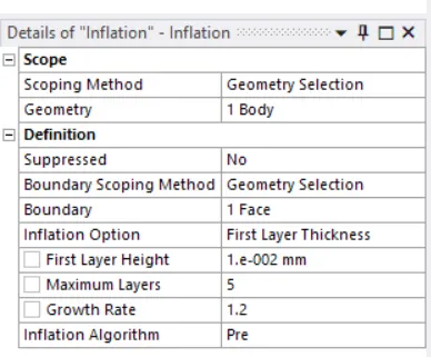
Inflation - Ahmed Body

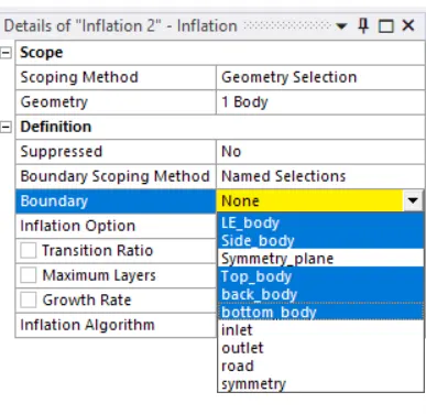
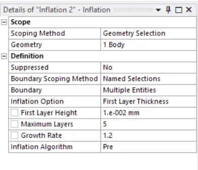
Even though the inflation layers were assigned with calculated first layer height, it is not visible because of the maximum number of elements limitations in the student version. But the inflation layer around the ahmed body & above road surface will be reuired to get the accurate results.

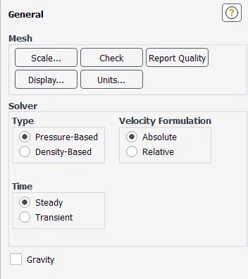
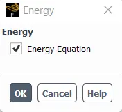
Simulation Setup:

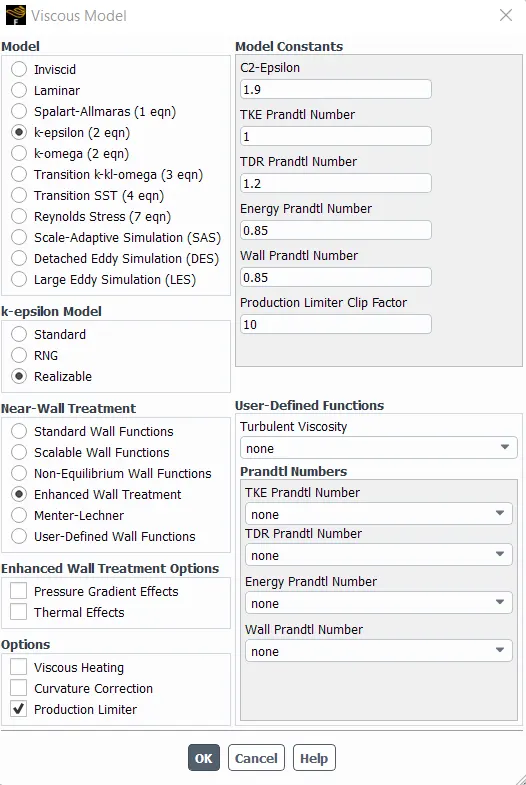
In viscous moel, k-epsilon model has been used with Realizable model & enhanced waal treatment.

The "production limiter" has also been activated which will handle & control any erratic conversion issue occur during simulation.

Material

Inlet

Road BC:

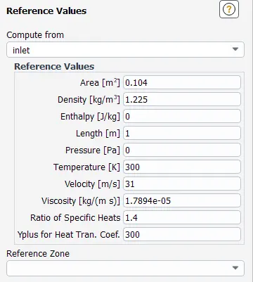
Reference Values

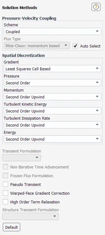
Solution Methods

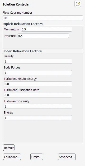
Solution Controls

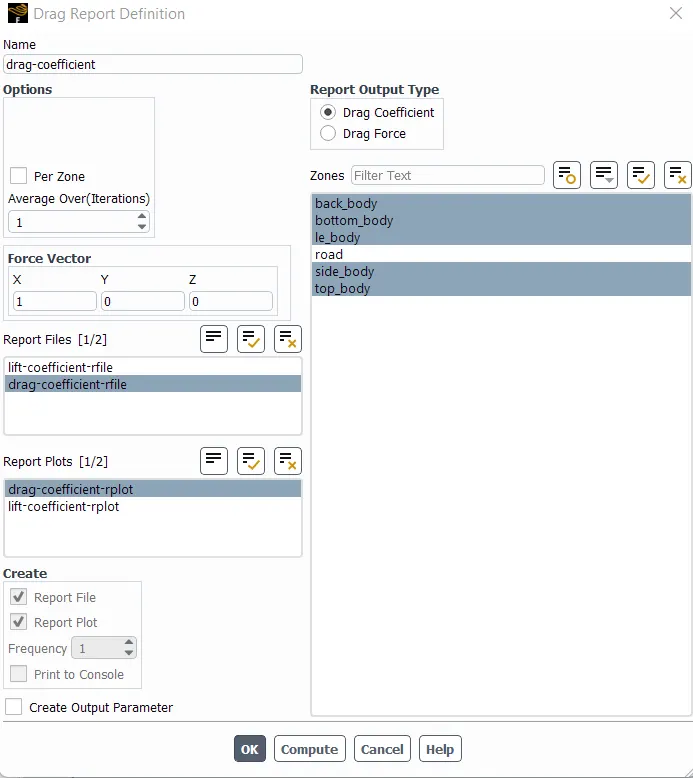
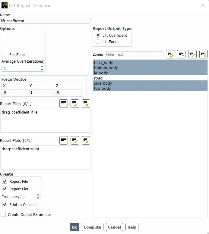
Report Definitions

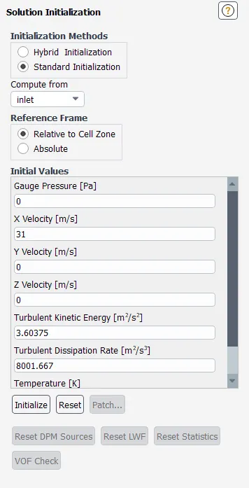
Solution Initialization

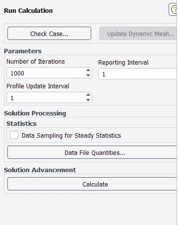
Part 3: Run the setup till convergence and plot for static pressure and coefficient of drag and lift to check for convergence

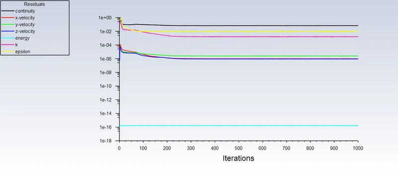
Residual Plot

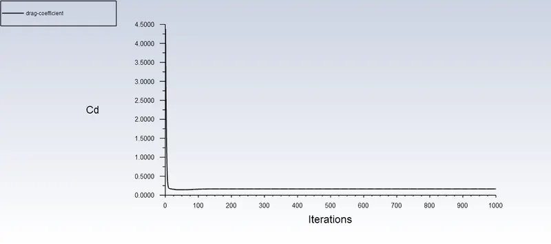
Drag Coefficient

Lift Coefficient

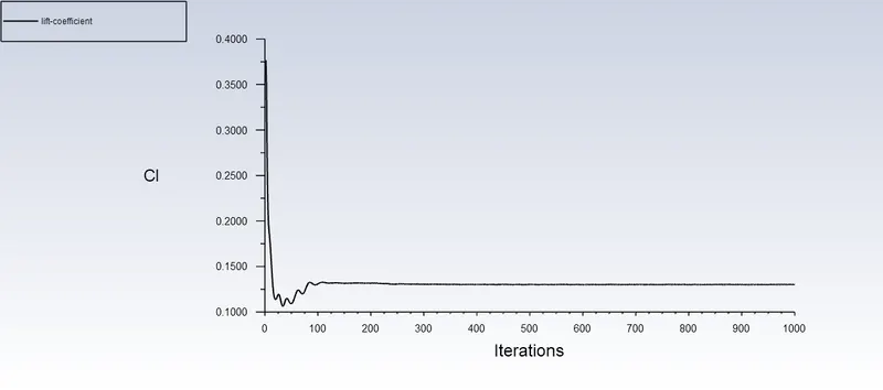
From the Residual plot & coefficient plots, it can be said that the solution is converged as values are neither fluctuating or increasing.

Pressure Contour

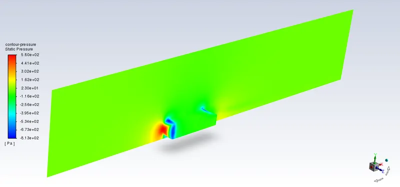
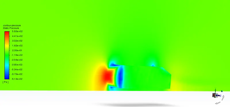
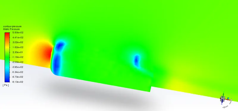
In the above static pressure plots, pressure variation is visible using contour plot. The blue region shows the dettachment of the flow from the body & Red color indicates the places where maximum pressure generated in the body. The blue color regions are the low pressure region.

Velocity Contour

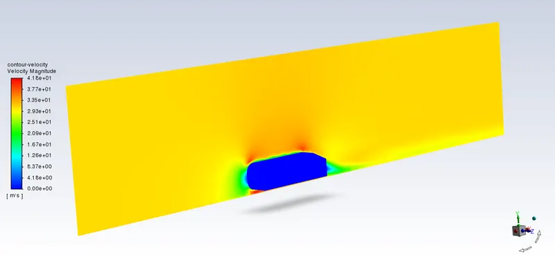
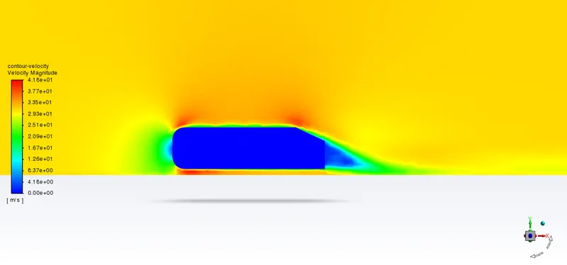
Part 4: Turn on Broadband- modelling and detail the acoustic field study over Ahmed body.

For Broadband modeling, the acoustics model needs to turn on using following option.

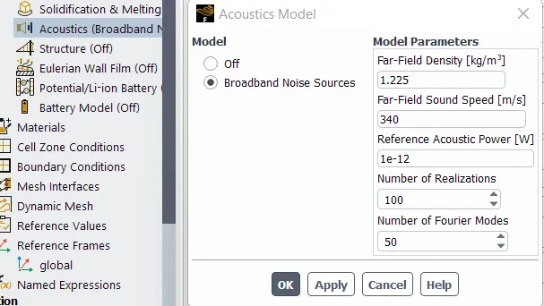
The number of Realization indicates that the number of samples which are going to use to solve the equation to determine the noise source term. The more number of realization involve than more numner of calculations will be solved.

After turning on Acoustics model, the software will calculate the noise source terms from already calculated results. The following contour plots can be used to determine the noise regions in Ahmed body.

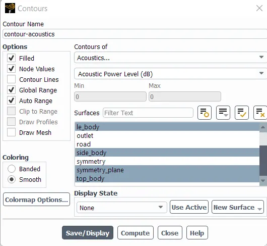
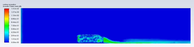
Below images of Acoustics Power level shows the region where the noise presents with higher desibel level. The wake region has maximum area which is responsible for creating noise.

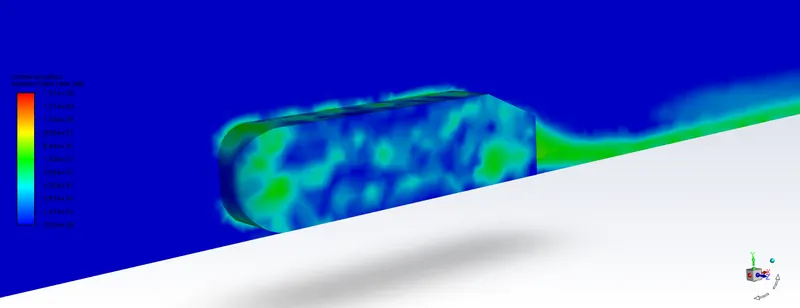
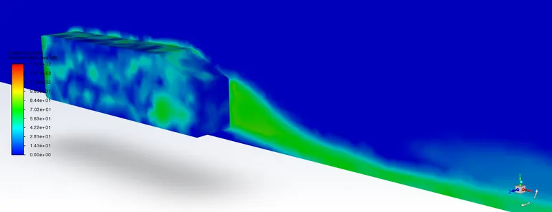
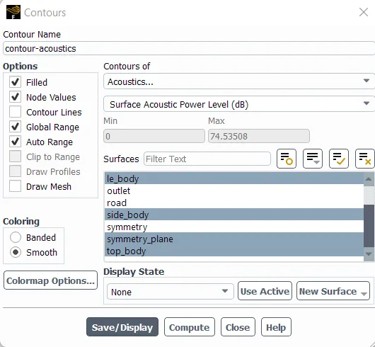
Using Surface Acoustics Power level plot, it will be easier to find the surfaces from where the noise has been generated because of aerodynamic forces.

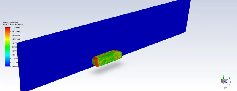
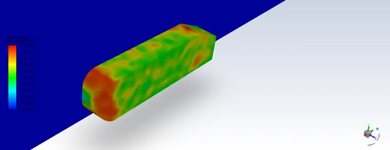
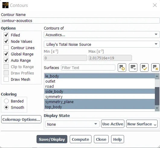
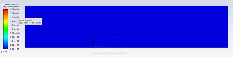
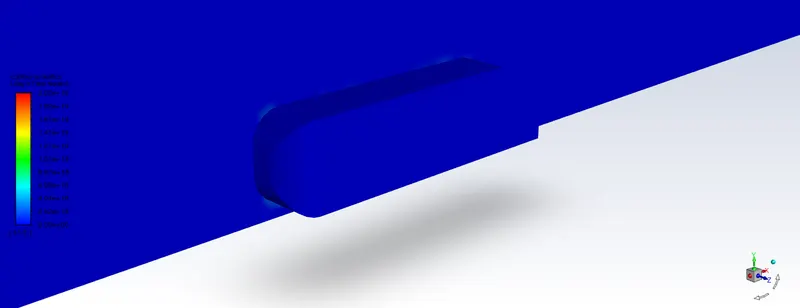
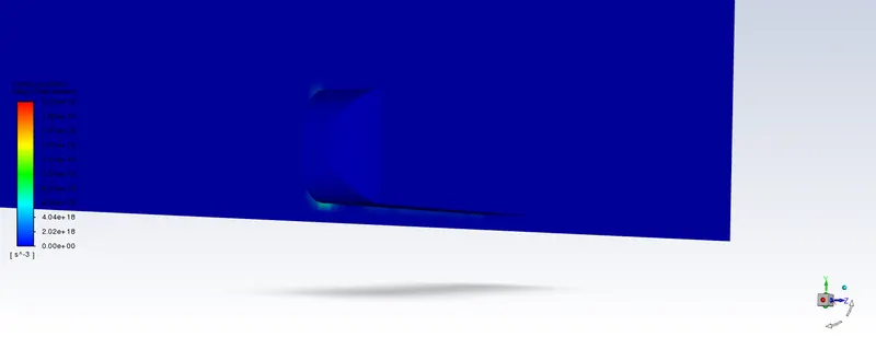
The Lilley's Total noise Source is used to find the noise sources. In case of Ahmed body, source term was determined at three places. One is at the end of windshield, second in below the frontal region of the body & third is where the flow is getting seperated from the body, at the end of roof.