Week 10 - Validation studies of Symmetry BC vs Wedge BC in OpenFOAM vs Analytical H.P equation
The aim of this challenge is to explore the application of the 'wedge' and the 'symmetry' boundary conditions to the simulation of a flow through a pipe. This is a continuation from the previous challenge with most of the basic set-up remaining the same.
The only differences incorporated in the basic set-up is that the length of the pipe is now reduced to 2 times the entrance length. This was done priomarily to ease the computational effort for performing the simulation due to the fewer number of cells (from 1000 to 800 cells in the 'x' direction). This also implies that the end time of our simulation can also be set proportionally lower ( to 8 seconds from 10 seconds). These changes were made in the 'blockMeshDict' files and the'controlDict' files respectively.
As we are mostly interested in the how the parameters vary along the length and the diameter of the pipe, the number of cells along the 'z' direction will remain '1' for all the angles.
The differnce between the 'wedge' and the 'symmetry' BCs:
The wedge boundary conditions is used specifically for cases with cylindrical or spherical symmetry. It involves a coordinate transformation and solves the governing equations in the cylindrical coordinate system. The symmetry boundary condition solves the governing equation in the cartesian plane itself. This boundary condition simply mirrors the results across the direction of symmtery. The symmerty boundary conditions is more general in its application unlike the wedge boundary condition, which is only restriced to cases of cylindrical or spherical symmetry.
A MATLAB code was written to automate the process of generating the 'blockMeshDict' script file. This made the process of generating the geomteries of all the different cases much more efficient:(The code, and consequently the script file itself, is common to all cases except for the inputs for the wedge angles and the boundary conditions at the front and the back faces.)
close all
clear
clc
%Pipe parametres:
Re=2100;
theta=10/25/45; %input for the wedge angle
d=0.004; r=(1/2)*d; L=2*0.05*Re*d;Le=0.05*Re*d; %The total length is taken as 2 times the entrance length.
%Fluid data:
rho=997; mu=8.9*10^-4;
Vavg=Re*mu/(rho*d);
Umax=2*Vavg;
%Vertices:
v0=[0 0 0];
v1=[0 r*cosd(theta/2) r*sind(theta/2)];
v2=[0 r*cosd(theta/2) -r*sind(theta/2)];
v3=[L 0 0];
v4=[L r*cosd(theta/2) r*sind(theta/2)];
v5=[L r*cosd(theta/2) -r*sind(theta/2)];
%BlockMesh parameters:
nx=800;
ny=15;
nz=1;
dimx=L/nx;dimy=r/ny;
arc_f=[1 2]; arc_b=[4 5];
========= |
\\ / F ield | OpenFOAM: The Open Source CFD Toolbox
\\ / O peration | Website: https://openfoam.org
\\ / A nd | Version: 9
\\/ M anipulation |
\*---------------------------------------------------------------------------*/
FoamFile
{
format ascii;
class dictionary;
object blockMeshDict;
}
// * * * * * * * * * * * * * * * * * * * * * * * * * * * * * * * * * * * * * //
convertToMeters 1;
vertices
(
(0 0 0)
(0 1.992389e-03 1.743115e-04)
(0 1.992389e-03 -1.743115e-04)
(8.400000e-01 0 0)
(8.400000e-01 1.992389e-03 1.743115e-04)
(8.400000e-01 1.992389e-03 -1.743115e-04)
);
blocks
(
hex (0 3 5 2 0 3 4 1) (800 15 1) simpleGrading (1 1 1)
);
edges
(
arc 1 2 (0 2.000000e-03 0)
arc 4 5 (8.400000e-01 2.000000e-03 0)
);
boundary
(
inlet
{
type patch;
faces
(
(0 1 2 0)
);
}
outlet
{
type patch;
faces
(
(3 5 4 3)
);
}
frontFace
{
type wedge/symmetry;
faces
(
(0 3 4 1)
);
}
backFace
{
type wedge/symmetry;
faces
(
(0 2 5 3)
);
}
topFace
{
type wall;
faces
(
(1 4 5 2)
);
}
axis
{
type empty;
faces
(
(0 3 3 0)
);
}
);
mergePatchPairs
(
);
// ************************************************************************* //
The 'controlDict' file that takes the inputs for setting up the simulation itself: (common to all cases.)
/*--------------------------------*- C++ -*----------------------------------*\
========= |
\\ / F ield | OpenFOAM: The Open Source CFD Toolbox
\\ / O peration | Website: https://openfoam.org
\\ / A nd | Version: 9
\\/ M anipulation |
\*---------------------------------------------------------------------------*/
FoamFile
{
format ascii;
class dictionary;
location "system";
object controlDict;
}
// * * * * * * * * * * * * * * * * * * * * * * * * * * * * * * * * * * * * * //
application icoFoam;
startFrom startTime;
startTime 0;
stopAt endTime;
endTime 8;
deltaT 0.0001;
writeControl timeStep;
writeInterval 2000;
purgeWrite 0;
writeFormat ascii;
writePrecision 6;
writeCompression off;
timeFormat general;
timePrecision 6;
runTimeModifiable true;
// ************************************************************************* //
Initail conditions for the set-up are defined in the script files that are in the '0' folder (also, common to all the cases exept for the BC for the front and the back faces.):
For 'U':
/*--------------------------------*- C++ -*----------------------------------*\
========= |
\\ / F ield | OpenFOAM: The Open Source CFD Toolbox
\\ / O peration | Website: https://openfoam.org
\\ / A nd | Version: 9
\\/ M anipulation |
\*---------------------------------------------------------------------------*/
FoamFile
{
format ascii;
class volVectorField;
object U;
}
// * * * * * * * * * * * * * * * * * * * * * * * * * * * * * * * * * * * * * //
dimensions [0 1 -1 0 0 0 0];
internalField uniform (0 0 0);
boundaryField
{
inlet
{
type fixedValue;
value uniform (0.4687 0 0);
}
outlet
{
type zeroGradient;
}
frontFace
{
type wedge/symmetry;
}
backFace
{
type wedge/symmetry;
}
topFace
{
type noSlip;
}
axis
{
type empty;
}
}
// ************************************************************************* //
For 'p':
/*--------------------------------*- C++ -*----------------------------------*\
========= |
\\ / F ield | OpenFOAM: The Open Source CFD Toolbox
\\ / O peration | Website: https://openfoam.org
\\ / A nd | Version: 9
\\/ M anipulation |
\*---------------------------------------------------------------------------*/
FoamFile
{
format ascii;
class volScalarField;
object p;
}
// * * * * * * * * * * * * * * * * * * * * * * * * * * * * * * * * * * * * * //
dimensions [0 2 -2 0 0 0 0];
internalField uniform 0;
boundaryField
{
inlet
{
type zeroGradient;
}
outlet
{
type fixedValue;
value uniform 0;
}
frontFace
{
type wedge/symmetry;
}
backFace
{
type wedge/symmetry;
}
topFace
{
type zeroGradient;
}
axis
{
type empty;
}
}
// ************************************************************************* //
In the 'constant' folder, we find the scrpit file for 'transportProperties'. There, we input the value for the kinematic presure:(common to all the cases)
/*--------------------------------*- C++ -*----------------------------------*\
========= |
\\ / F ield | OpenFOAM: The Open Source CFD Toolbox
\\ / O peration | Website: https://openfoam.org
\\ / A nd | Version: 9
\\/ M anipulation |
\*---------------------------------------------------------------------------*/
FoamFile
{
format ascii;
class dictionary;
location "constant";
object transportProperties;
}
// * * * * * * * * * * * * * * * * * * * * * * * * * * * * * * * * * * * * * //
nu [0 2 -1 0 0 0 0] 8.917e-7;
// ************************************************************************* //
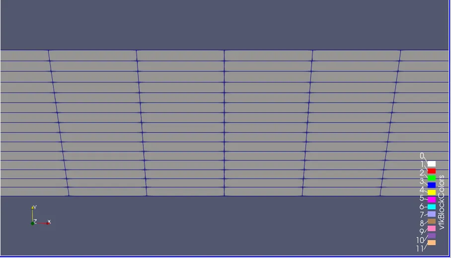
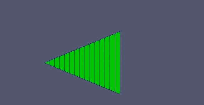
Generated Meshes:
`10^o`:
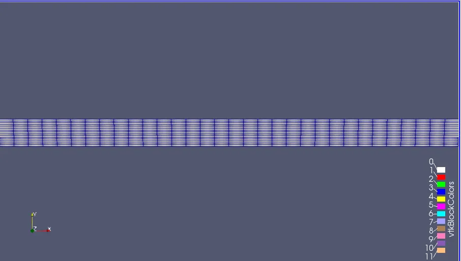
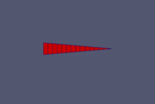
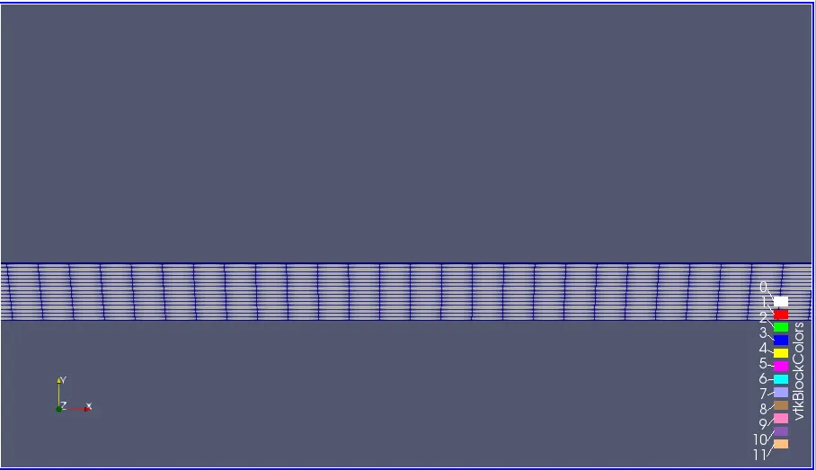
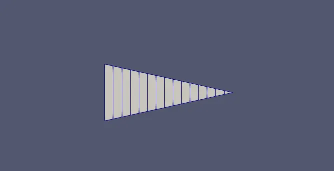
`25^o`:
`45^o`:
Analyitical Results:
For the 'Entrance Length':
The entrance length is calculated as:
`Le=0.05*Re*D`
From the above equation we get the value of the entrance length to be 0.42m.
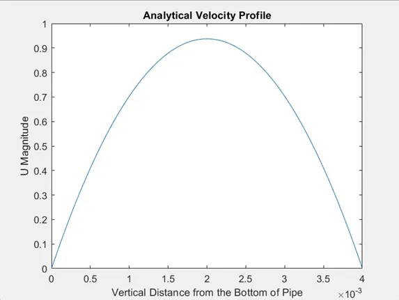
For the velocity profile:
The general equation describing the velecity profile for the fully developed region is:
`2*U_(avg)*(1-(r/R)^2)`
Also,
`U_(max)=2*U_(avg)=0.9374m/s`.
A code has been written in MATLAB to generate this profile,
close all
clear
clc
mu=8.9*10^-4;
x=linspace(0,0.004);
y=0.9374*(1-((x-0.002).^2)/0.002^2);
figure (1)
plot(x,y)
title('Analytical Velocity Profile')
xlabel('Vertical Distance from the Centre to Top')
ylabel('U Magnitude')
Pressure Drop:
The Hagen-Poiseuille Equation has been used to calculate the analytical pressure drop across the developed region.
Q=`(DeltaP*pi*r^4)/(8*mu*L)`
A MATLAB code has been written to calculate the analytical pressure-drop:
close all
clear
clc
The obtained value for the pressure drop is 350.3672 Pascals.
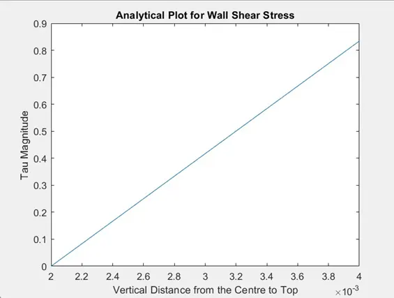
For Wall Shear Stress:
Wall shear stress can be calculated by:
`tau=-mu((delU)/(dely))`
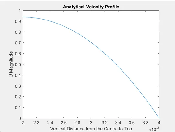
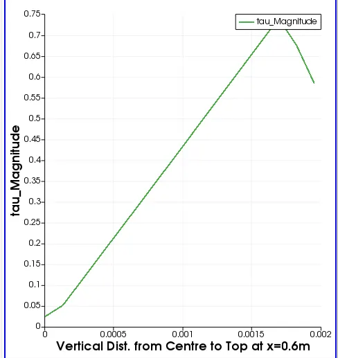
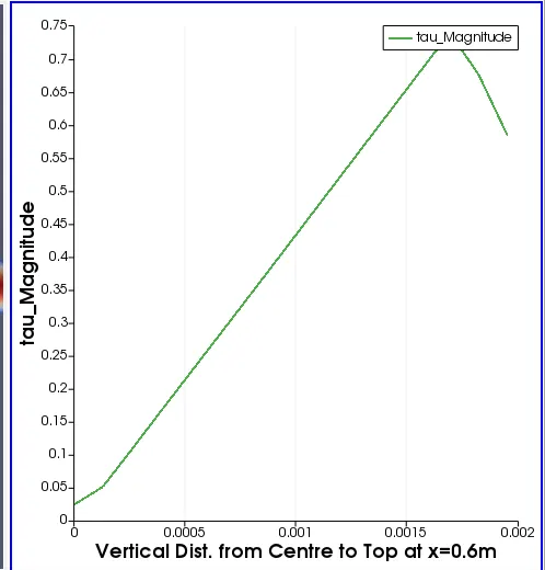
On substituing the analytical expression for the velocity profile, we can obtain the profile for the wall shear stress.
Wall shear stress has been calculated and plotted using the below MATLAB code.
close all
clear
clc
mu=8.9*10^-4;
x=linspace(0.002,0.004);
y=0.9374*(1-((x-0.002).^2)/0.002^2);
tau=(2*0.9373*(x-0.002)*mu)/0.002^2;
figure (1)
plot(x,y)
title('Analytical Velocity Profile')
xlabel('Vertical Distance from the Centre to Top')
ylabel('U Magnitude')
For `10^o`:
Wegde boundary condition,
Visualising the 'Entrance Length':
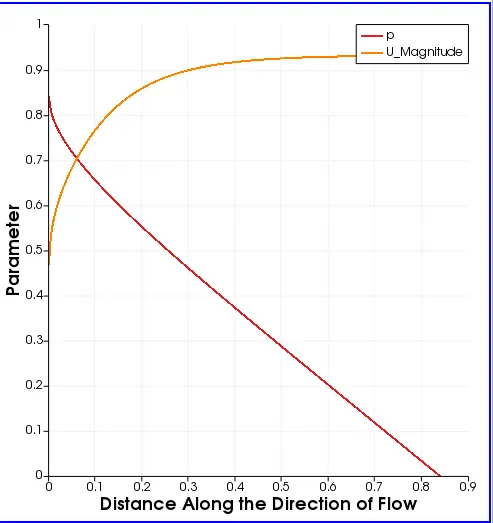
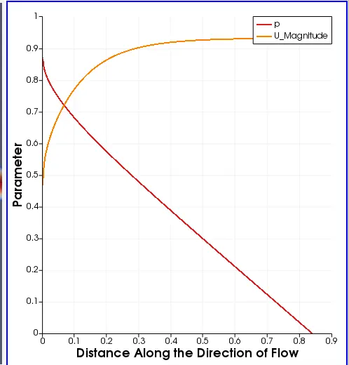
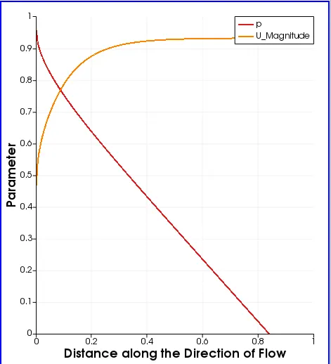
Clearly, the velocity becomes 'x' invariant and the pressure curve adopts a linear curve after '`x~~0.46`'. Thus, the entrance length is 'x=0.46m' which is close to the analytically calculated value.
Velocity Profile:
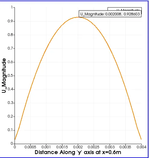
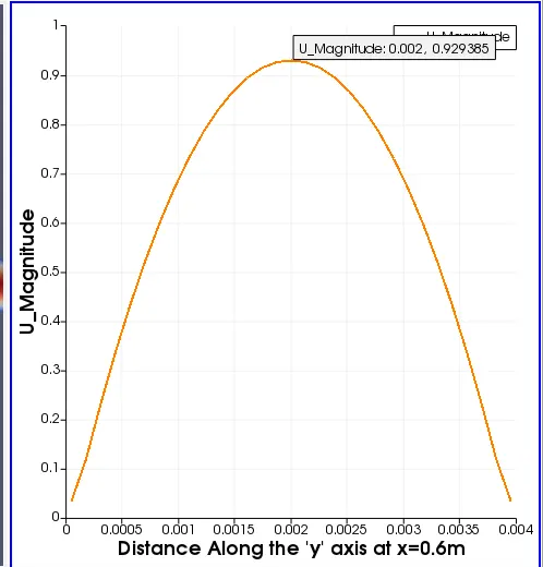
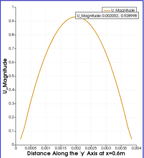
Velocity profile matches the analytical plot. Also, '`U_(max)~~0.928`' which is close to the analytically calculated value.
Pressure Drop:
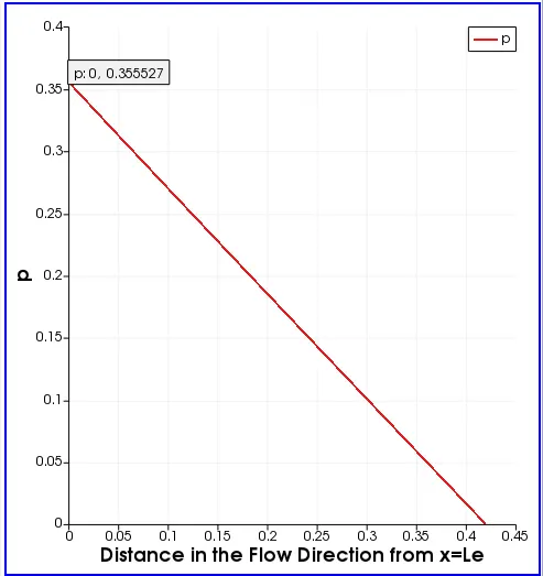
The pressure drop seen from the graph is `DeltaP=0.355527*997 Pascals=354.460Pascals` which is close to the analytically calculated value.
Wall Shear Stress:
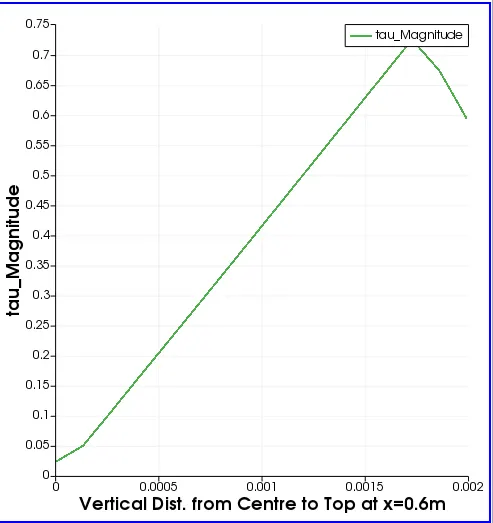
The obtained plot is similar to the analytical plot.
Symmetry BC:
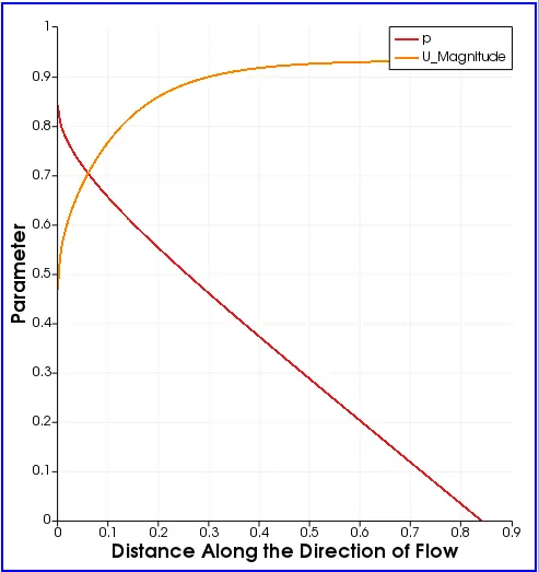
From the graph, the entrance length seems to be somewhere in the neighbourhood of x=0.46m. This is close to the analytical value. The plot obtained from the previous simulation with the wedge BC is nearly identical.
Velocity Profile:
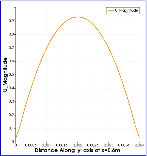
The obtained plot is simmilar to the analytical plot from MATLAB. Also the value if '`U_(max)`' seen from the graph is close to the analytical value. The velocity profiles obtained from the simulation run with the wedge BC is very similar to the one obtained from the simulation run with the symmetry BC.
Pressure Drop:
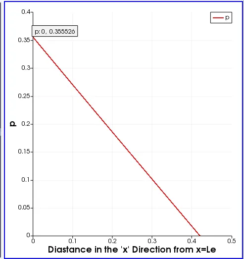
The pressure drop across the developed region obtained from the simulation (354.46 Pascals) is very close to what was calculated from the Hagen-Poiseuille Equation (350.3672 Pascals). It can also be seen that the value of the pressure drop obtained from the simulation with the wedge boundary condition is also the effectively the same.
Wall Shear Stress:
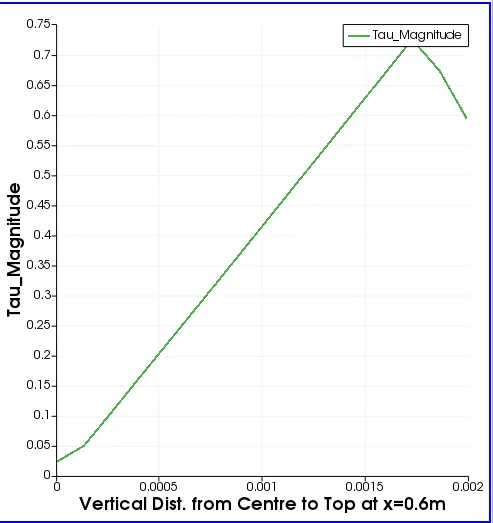
The plot is similar to the analytically derived plot and also to the plot obtained from the previous simulation.
Thus, a trend of very similar results and plots were observed from both the simulations despite the different BCs applied on the front and the back faces.
This regime of similarity was obtained for not just for the different BCs but for different wedge angles as well.
For `25^o`,
For Wedge BC:
Visualising the 'Entrance Length':
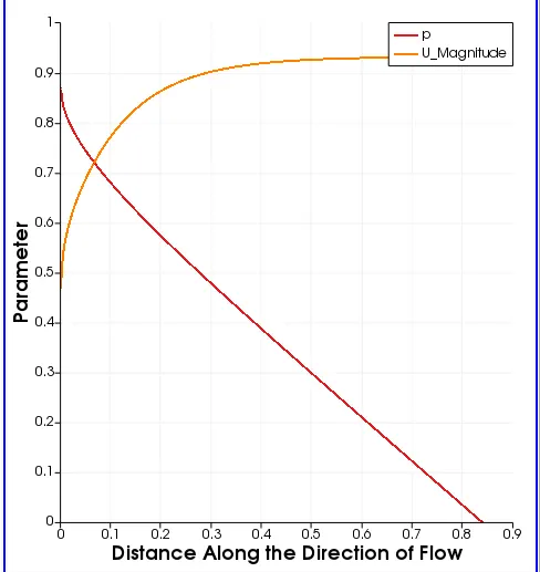
Velocity Profile:
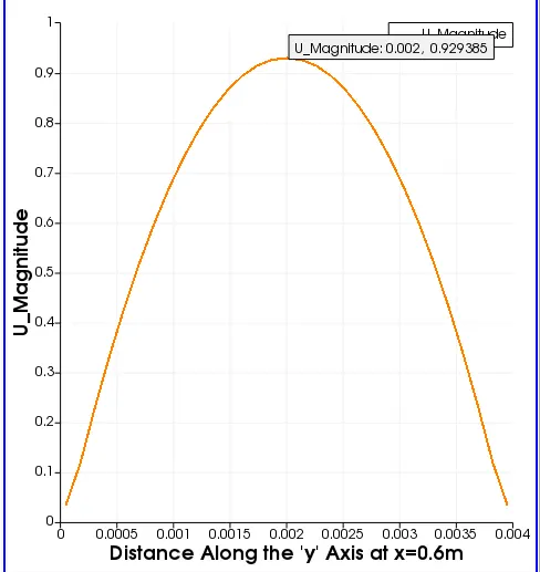
Pressure Drop:
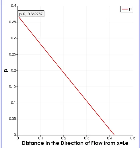
(Calculated value of Pressure drop from the simulation is 368.64773 Pascals.)
Wall Shear Stress:
For Symmetry BC:
Visualising the 'Entrance Length':
Velocity Profile:
Pressure Drop:
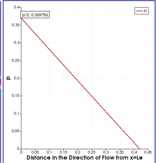
(Calculated value of Pressure drop from the simulation is 368.64673 Pascals.)
Wall Shear Stress:
For `45^o`:
For Wedge BC:
Visualising the 'Entrance Length':
Velocity Profile:
Pressure Drop:
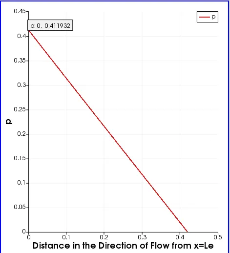
(Calculated value of Pressure drop from the simulation is 410.696204 Pascals.)
Wall Shear Stress:
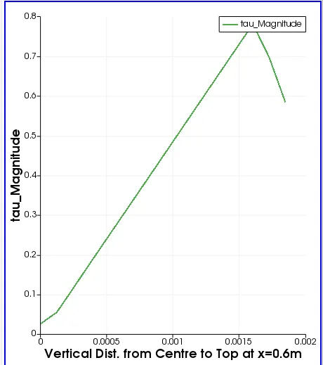
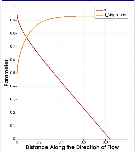
For Symmetry BC:
Visualising the 'Entrance Length':
Velocity Profile:
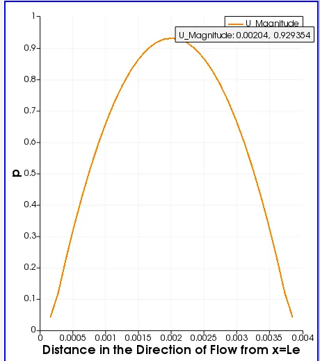
Pressure Drop:
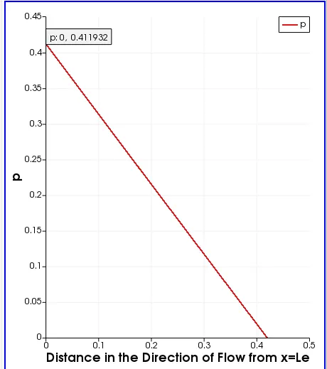
(Calculated value of Pressure drop from the simulation is 410.696204 Pascals.)
Wall Shear Stress:
[The script files for the case with '`10^o`' wedge angle have been appended along with the MATLAB codes.]