Week 10 - Simulation of Flow through a pipe in OpenFoam
The aim of this challenge is to simulate an axisymmetric flow through a pipe where the geometry definition is automated by means of a MATLAB code that automates the generation of the ‘blockMeshDict’ file and to validate the obtained results with the Hagen-Poiseuille equation for a fully developed flow.
Description of the problem:
This simulation mainly studies the fully developed flow in a pipe. The primary characteristic of fully developed flows is the fact that the velocity profile remains constant along the flow. This implies that the velocity is invariant in the direction of the flow. A constant velocity profile also means that the velocity gradient at the walls is constant. Thus, we can say that another defining characteristic for a fully developed flow is the presence of a constant wall shear stress.
Also, in the fully developed region, the pressure forces are completely balanced out by the viscous forces. This implies that the inertia terms (the non-linearity inducing, complex terms) are absent in the governing equation for the momentum in the flow direction. Thus, we get a linear pressure profile along the flow in the region.
Another definition of fully developed flow is the region from where the boundary layers meet. The length of the ‘developing’ region where the boundary layers are yet to meet is called the ‘entrance length’. The boundary layer is the demarcation up to which the viscous effects of the wall can be felt (or alternatively, where a considerable amount of velocity gradient exists.) The boundary layer obviously extends from the wall towards the free stream. As we have walls on both the top and bottom, the boundary layers can only extend till the point where they meet. Thus, in the developing region (the region where the boundary layers have not yet merged), the inviscid core gets smaller and more constricted by the developing boundary layers. Thus, the fluid here accelerates to a maximum value which is reached when the boundary layers merge (as the fluid can then no longer accelerate).
The velocity profile is obviously not constant in the developing region. The inertia terms are also very much present in the momentum governing equation making the analysis in this regime quite difficult.
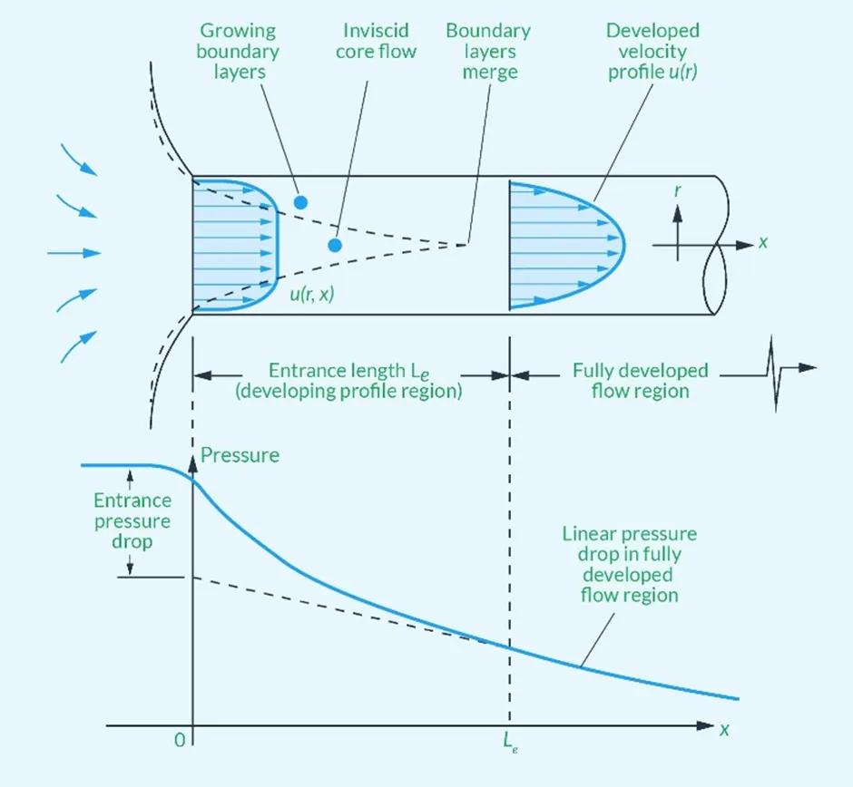
This linear pressure drop in the developed region is characterised by the Hagen-Poiseuille equation:
Q=`(DeltaP*pi*r^4)/(8*mu*L)`
(for laminar flow regimes.)
Here,
'Q' is the volume flow rate, '`DeltaP`' is the pressure drop, '`mu`' is the dynamic viscosity.
Data to be inputted:
Given: Inlet Reynold's number=2100.
Fluid used: Water at `25^o`C.
`rho=997kg/m^3`
`mu=0.0089 Pa*s`
Assumed diameter of the pipe=0.004m.
The length of the pipe was taken to be 2.5 times the entrance length 'Le'.
`Le~~0.05*Re*D` ...(i)
On calculating, 'Le=0.42m' and thus, 'entrance length=1.05m'.
We know, for internal flows, `Re=(rho*U_(avg)*D)/mu` ...(ii)
From (ii), we can calculate the value of '`U_(avg)`'.
`U_(avg)=(Re*mu)/(rho*D)`
`U_(avg)=0.4687m/s`
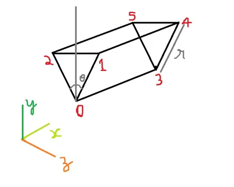
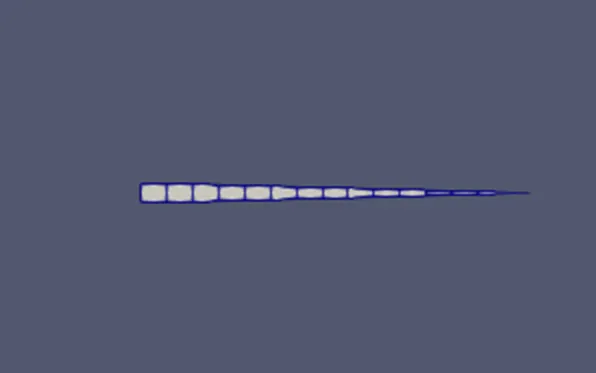
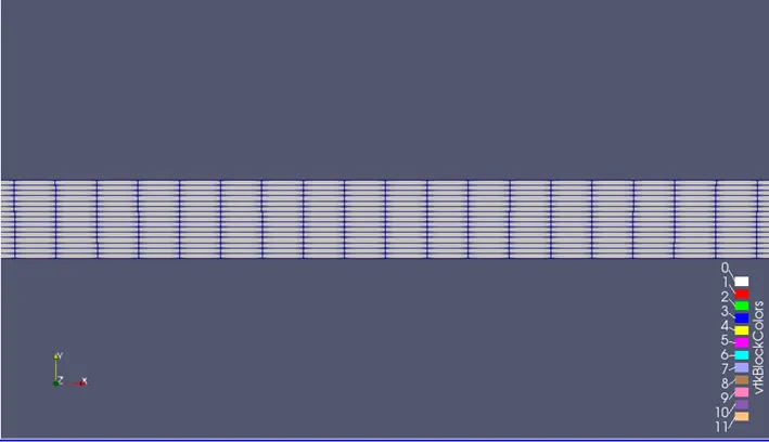
Since running this simulation is computationally intensive, we only simulate the flow through a tiny wedge section of the actual pipe (with sector angle as '`3^o`'). This can be done as the flow is axisymmetric, meaning that rotational symmetry exists along with the condition of zero whirl component.
A MATLAB code was written to automate the process as necessary changes could be required to the geometry, number of cells, etc. to make the simulation efficient.
MATLAB CODE:
close all
clear
clc
%Pipe parametres:
Re=2100;
theta=3;
d=0.004; r=(1/2)*d; L=2.5*0.05*Re*d;Le=0.05*Re*d; %The total length is taken as 2.5 times the entrance length.
%Fluid data:
rho=997; mu=8.9*10^-4;
Vavg=Re*mu/(rho*d);
Umax=2*Vavg;
%Vertices:
v0=[0 0 0];
v1=[0 r*cosd(theta/2) r*sind(theta/2)];
v2=[0 r*cosd(theta/2) -r*sind(theta/2)];
v3=[L 0 0];
v4=[L r*cosd(theta/2) r*sind(theta/2)];
v5=[L r*cosd(theta/2) -r*sind(theta/2)];
%BlockMesh parameters:
nx=1000;
ny=15;
nz=1;
dimx=L/nx;dimy=r/ny;
arc_f=[1 2]; arc_b=[4 5];
Resulting 'blockMeshDict' file:
/*--------------------------------*- C++ -*----------------------------------*\
========= |
\\ / F ield | OpenFOAM: The Open Source CFD Toolbox
\\ / O peration | Website: https://openfoam.org
\\ / A nd | Version: 9
\\/ M anipulation |
\*---------------------------------------------------------------------------*/
FoamFile
{
format ascii;
class dictionary;
object blockMeshDict;
}
// * * * * * * * * * * * * * * * * * * * * * * * * * * * * * * * * * * * * * //
convertToMeters 1;
vertices
(
(0 0 0)
(0 1.999315e-03 5.235390e-05)
(0 1.999315e-03 -5.235390e-05)
(1.050000e+00 0 0)
(1.050000e+00 1.999315e-03 5.235390e-05)
(1.050000e+00 1.999315e-03 -5.235390e-05)
);
blocks
(
hex (0 3 5 2 0 3 4 1) (1000 15 1) simpleGrading (1 1 1)
);
edges
(
arc 1 2 (0 2.000000e-03 0)
arc 4 5 (1.050000e+00 2.000000e-03 0)
);
boundary
(
inlet
{
type patch;
faces
(
(0 1 2 0)
);
}
outlet
{
type patch;
faces
(
(3 5 4 3)
);
}
frontFace
{
type wedge;
faces
(
(0 3 4 1)
);
}
backFace
{
type wedge;
faces
(
(0 2 5 3)
);
}
topFace
{
type wall;
faces
(
(1 4 5 2)
);
}
axis
{
type empty;
faces
(
(0 3 3 0)
);
}
);
mergePatchPairs
(
);
// ************************************************************************* //
Geometry schematic:
Resulting Geometry:
(Frontal view.)
(A closer look from the side.)
Initial Conditions:
The initial conditions are set by making changes to the script files in the '0' folder. For velocity and pressure boundary conditions, if one is specified as a Neumann condition, the other must be specified as a Dirichlet condition and vice-versa.
For 'U':
/*--------------------------------*- C++ -*----------------------------------*\
========= |
\\ / F ield | OpenFOAM: The Open Source CFD Toolbox
\\ / O peration | Website: https://openfoam.org
\\ / A nd | Version: 9
\\/ M anipulation |
\*---------------------------------------------------------------------------*/
FoamFile
{
format ascii;
class volVectorField;
object U;
}
// * * * * * * * * * * * * * * * * * * * * * * * * * * * * * * * * * * * * * //
dimensions [0 1 -1 0 0 0 0];
internalField uniform (0 0 0);
boundaryField
{
inlet
{
type fixedValue;
value uniform (0.4687 0 0);
}
outlet
{
type zeroGradient;
}
frontFace
{
type wedge;
}
backFace
{
type wedge;
}
topFace
{
type noSlip;
}
axis
{
type empty;
}
}
// ************************************************************************* //
For 'p':
/*--------------------------------*- C++ -*----------------------------------*\
========= |
\\ / F ield | OpenFOAM: The Open Source CFD Toolbox
\\ / O peration | Website: https://openfoam.org
\\ / A nd | Version: 9
\\/ M anipulation |
\*---------------------------------------------------------------------------*/
FoamFile
{
format ascii;
class volScalarField;
object p;
}
// * * * * * * * * * * * * * * * * * * * * * * * * * * * * * * * * * * * * * //
dimensions [0 2 -2 0 0 0 0];
internalField uniform 0;
boundaryField
{
inlet
{
type zeroGradient;
}
outlet
{
type fixedValue;
value uniform 0;
}
frontFace
{
type wedge;
}
backFace
{
type wedge;
}
topFace
{
type zeroGradient;
}
axis
{
type empty;
}
}
// ************************************************************************* //
Changes were made to the 'controlDict' too. The time-step size was chosen to be 0.0001seconds to maintain a reasonable value of the Courant number (the smaller of the two mesh cell dimension was 0.000133m) .The 'writeInterval' was set to '2000' to accommodate such a large simulation with such a small time-step.
/*--------------------------------*- C++ -*----------------------------------*\
========= |
\\ / F ield | OpenFOAM: The Open Source CFD Toolbox
\\ / O peration | Website: https://openfoam.org
\\ / A nd | Version: 9
\\/ M anipulation |
\*---------------------------------------------------------------------------*/
FoamFile
{
format ascii;
class dictionary;
location "system";
object controlDict;
}
// * * * * * * * * * * * * * * * * * * * * * * * * * * * * * * * * * * * * * //
application icoFoam;
startFrom startTime;
startTime 0;
stopAt endTime;
endTime 10;
deltaT 0.0001;
writeControl timeStep;
writeInterval 2000;
purgeWrite 0;
writeFormat ascii;
writePrecision 6;
writeCompression off;
timeFormat general;
timePrecision 6;
runTimeModifiable true;
// ************************************************************************* //
Post Processing and Validation of Results:
Post-Processing:
Taking advantage of the fact that the flow is axisymmetric, the simulation was only done for a small wedge of the pipe to save on computational effort. As a result, we only get half of the profiles across a cross section for the various parameters that are under study.
Due to symmetrical geometry and boundary conditions about the axis, the results will also be symmetric. Thus the ‘reflect’ option could be used to obtain the complete geomtery.
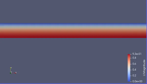
(Before using 'reflect'.)
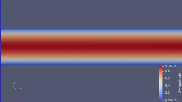
(Complete geometry obtained after using 'reflect'.)
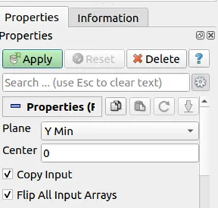
(Selecting the plane of symmetry for applying 'reflect'.)
Validation of 'Hydrodynamic Length':
The hydrodynamic entrance length (Le) is calculated as:
`Le~~0.05*Re*D` ...(from equation (i)).
On inputting the values, we get the entrance length to be 0.42m.
We can validate this to be the entrance length by observing the velocity profile in the flow direction obtained from the performed simulations.
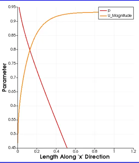
From around 'x=0.42m' the velocity becomes constant ('x' invariant) and the pressure curve attains a linear nature. This indicates that the fully developed zone starts from around 'x=0.42m' , thus making the entrance length, 'Le=0.42m'.
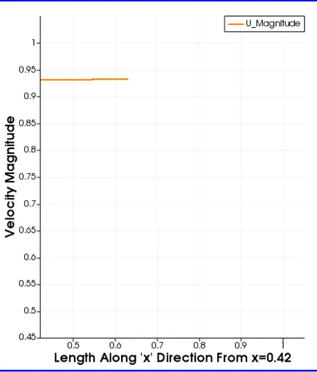
(From 'x=0.42m onwards, the velocity magntude is parallel to the 'x'-axis.)
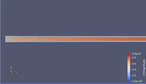
(Visualising the entrance length from the obtained contours.)
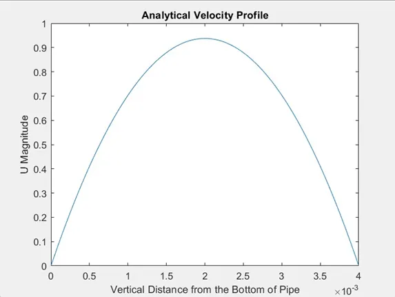
Validation of the fully developed velocity profile:
The general velocity profile (for laminar regime) of the fully developed flow is given:
`u(r)=U_(max)*(1-(r/R)^2)` ...(iii)
Where, 'R' is the radius of the pipe and 'r' is the radial distance.
Here, `U_(max)=2*U_(avg)` ...(iv)
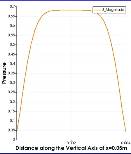
(Velocity profile in the developing region obtained from the simulation.)
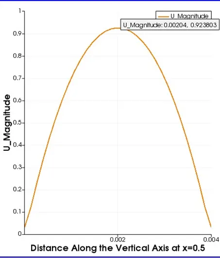
(Velocity profile in the developed region obtained from the simulation.)
Validation of the Pressure Plot using the Hagen-Poiseuille Equation:
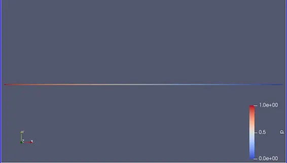
(Pressure variation visualised through contours obtained from the simulation.)
Q=`(DeltaP*pi*r^4)/(8*mu*L)`
using this, calculating the pressure drop `DeltaP=525.5508` Pascals.
MATLAB code for the above calculation:
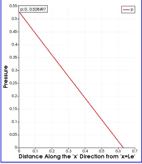
(Plot of pressure variation along the flow direction obtained from the simualtion.)
From the graph we can see that the drop in kinematic pressure is 0.528497 `m^2/s^2`.
we know, kinematic pressure`*`fluid density `(997kg/m^3)`=pressure in Pascals.
Thus, the pressure drop obtained from the simualtion is 528.497 Pascals.
Validation of Wall Shear Stress calculations:
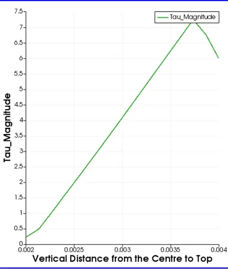
(Plot obtained from the simulation.)
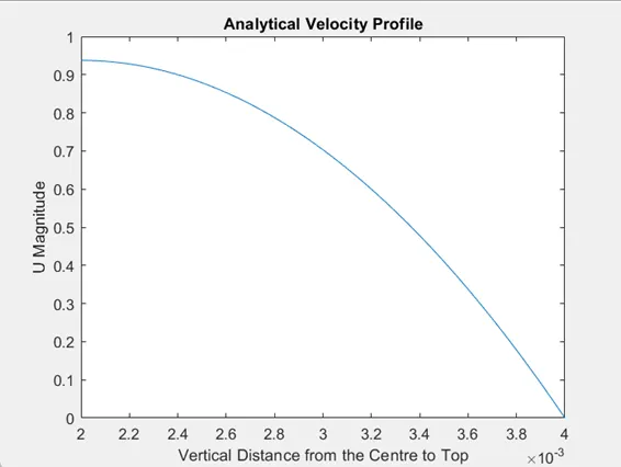
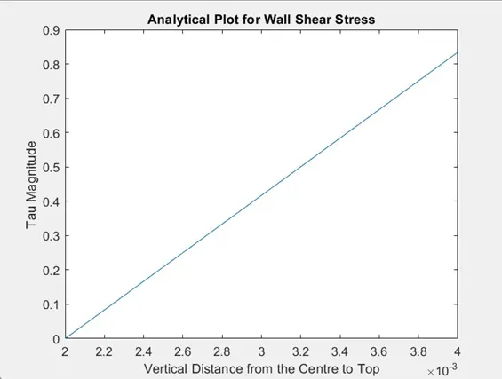
(Analytically derived.)
The similarity in both plots is visible.