Week 10 - Simulating Combustion of Natural Gas.

Challenge 10 – Simulating the combustion of NATURAL GAS (methane)

Aim – To analyse the emissions and calculate the mass fraction of species resulting from the combustion of natural gas

Introduction to Combustion of natural gas –

Natural Gas is a naturally-occurring mixture of hydrocarbon and non-hydrocarbon gases found in porous formations beneath the earth's surface. It is not a pure element like oxygen, but a mixture of gases of which hydrocarbon gases are the components that are combustible and produce heat.

Natural gas distributed by utilities varies in composition. The heat-producing hydrocarbons are composed of the elements Carbon and Hydrogen. Methane (CH4) is always the largest component. Ethane, propane (C3H8) and butane are heavier, "hotter" hydrocarbons produced from natural gas wells, and are present in low concentration. Nitrogen, Oxygen, and Carbon Dioxide are the major components (99.9%) of air, but are considered contaminants of natural gas.

Combustion of natural gas is the chemical reaction of oxygen with a combustible material which produces heat.

There are three requirements for combustion. If one of these three components is missing, combustion cannot occur.

• Fuel (natural gas, in this case).
• Oxygen.
• A source of ignition.

Natural gas will not burn unless the mixture is within a flammable range of roughly 4 to 15% gas per volume of air. Above and below, these amounts it will not burn. The most efficient or ideal mixture is about 10% gas.

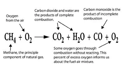
Geometry modelling-

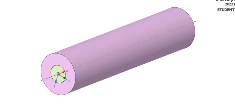
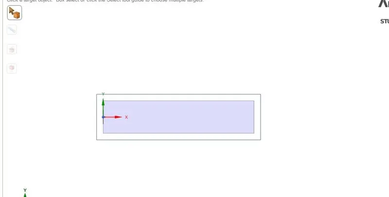
2D Geometry

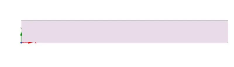
Meshing –

Statistics:

Number of nodes=107053

Number of elements=105933

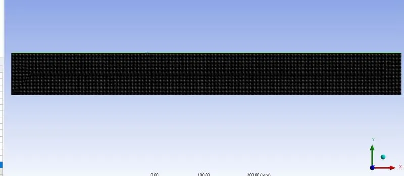
Named sections:

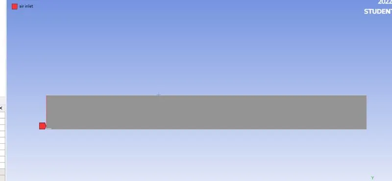
Air inlet

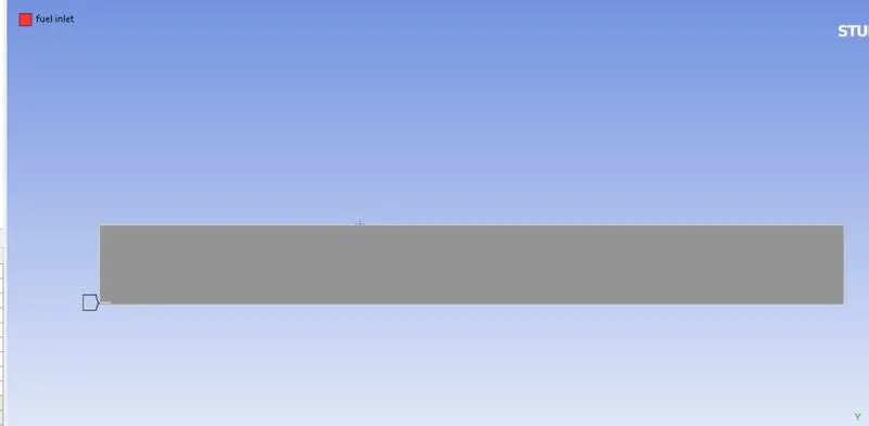
Fuel inlet

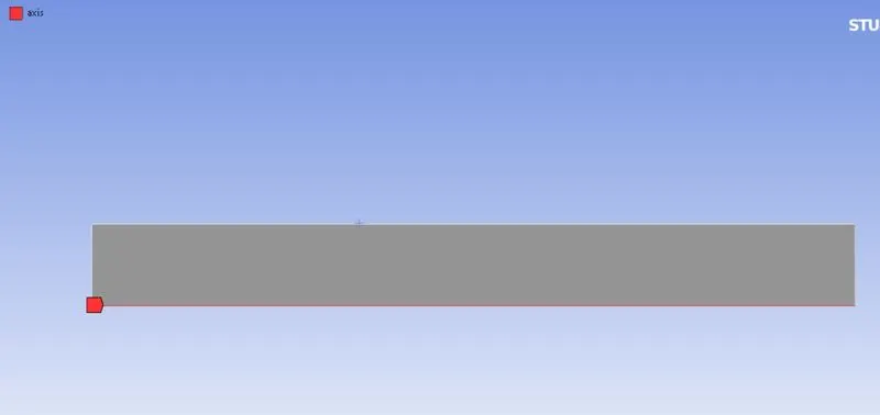
Axis

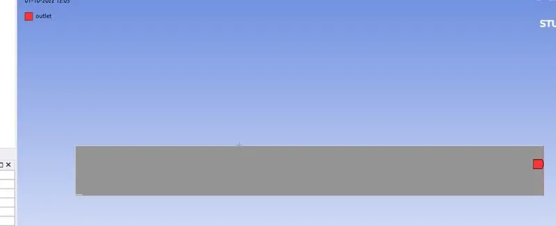
Outlet

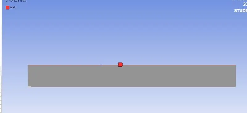
Walls

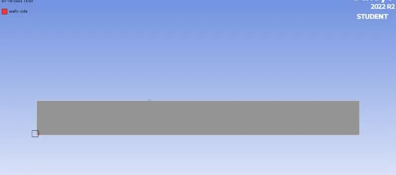
Walls-side

Setting up the case in Ansys Setup –

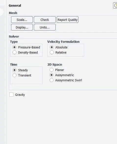
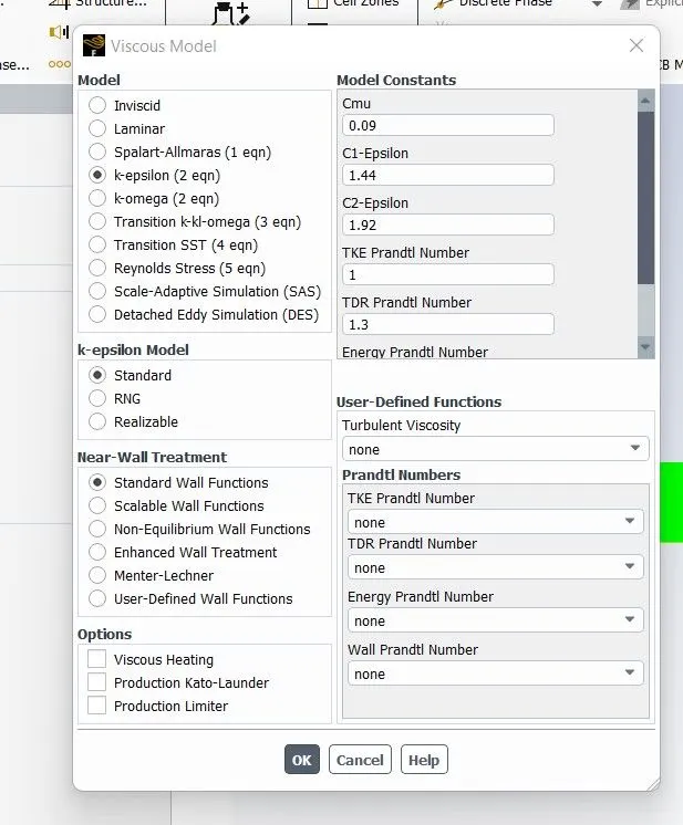
1. Firstly, in Ansys fluent setup, the pressure-based model was chosen since we are dealing with velocities less than 0.3 times the speed of sound.
2. In that case, it is advisable to choose a density-based model
3. Furthermore, a steady state solver was used since only the end results needed to be observed
4. Most importantly, the 2D space was given as “axisymmetric” without which the simulation will not give proper results.
5. Since this particular problem does not deal with wall related properties, a k-epsilon standard wall functions model was used rather than a k-omega SST model.
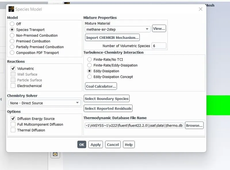
6. The species transport equation was turned on and the following conditions were used

• Reactions – volumetric
• Options – inlet diffusion and diffusion energy source
• Mixture material – methane air – 2 steps
• Turbulence chemistry interaction – eddy dissipation
• Number of volumetric species – 6

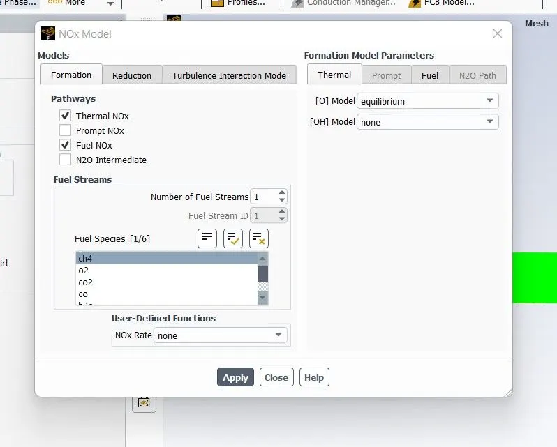
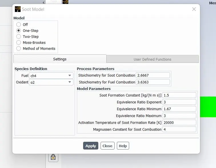
7. Furthermore, the NOx and SOOT model were turned on to observe the emissions at the outlet
8. Thermal NOx pathway was used and a one-step SOOT model was used for analysis
9. Boundary conditions –

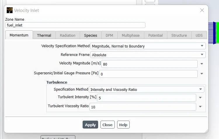
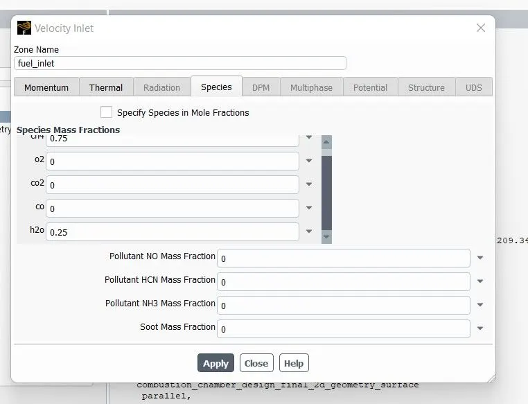
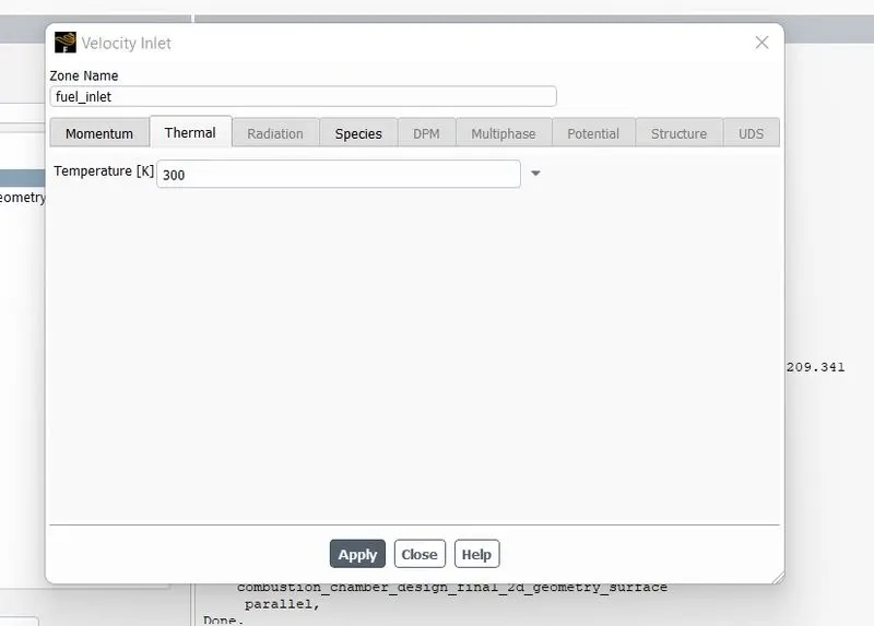
• Fuel inlet –
  1. Velocity inlet = 80m/s
  2. Temperature = 300K

• Species – CH4 = 1 mass fraction, and water = 0 mass fraction

1. The mass fraction of water and CH4 was altered according to each iteration base on the amount of water mixed with methane

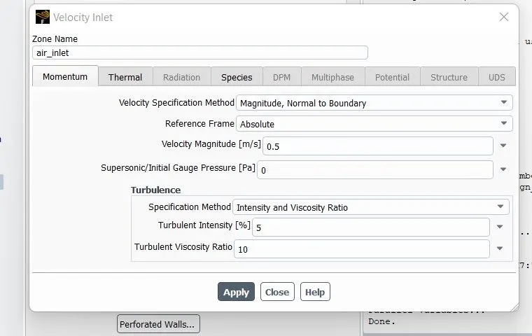
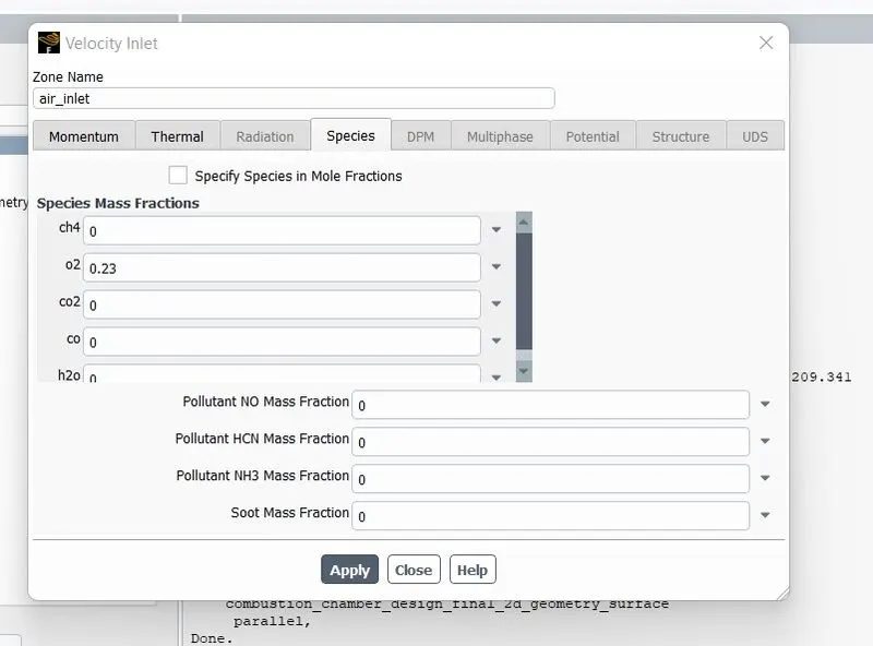
• Air inlet –

1. Velocity inlet = 0.5m/s
2. Temperature = 300K

• Species – O2 – 0.23 mass fractionFinally the solution was initialised using hybrid initialisation and run for 600 iterations.

10. Finally the solution was initialised using hybrid initialisation and run for 600 iterations.

Results and Findings –

1.0% WATER-100% NATURAL GAS

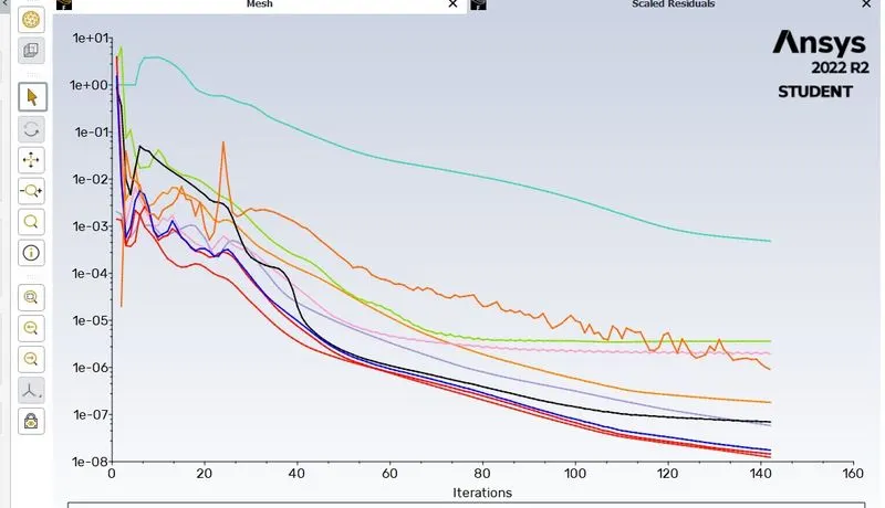
2.5% WATER-95% NATURAL GAS

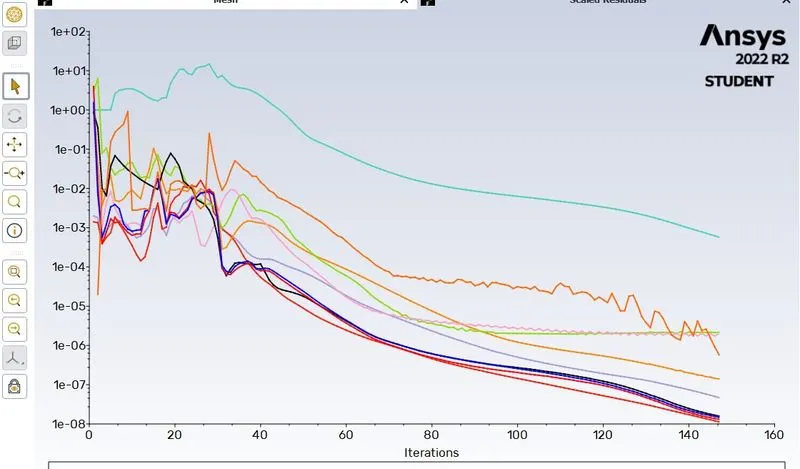
3.10% WATER-90% NATURAL GAS

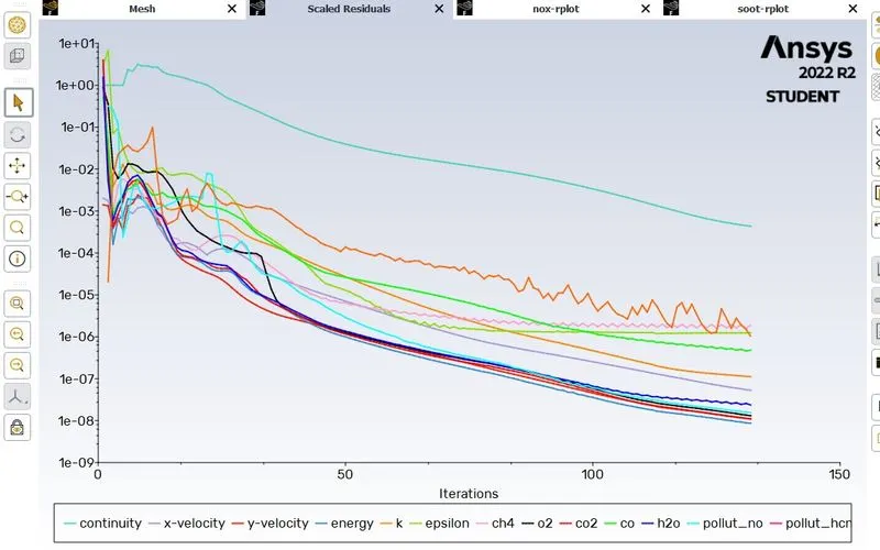
4.15% WATER-85% NATURAL GAS

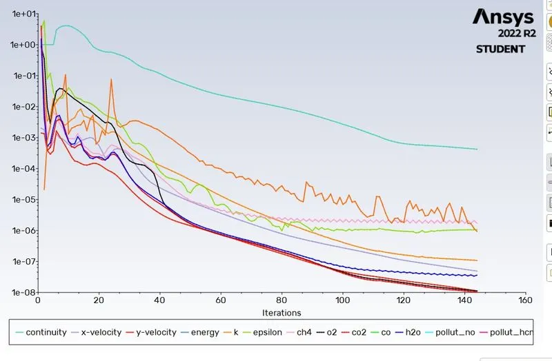
5.20% WATER-80% NATURAL GAS

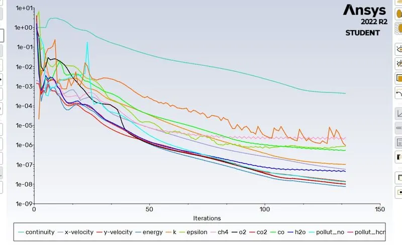
6.25% WATER-75% NATURAL GAS

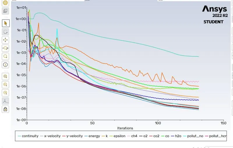
7.30% WATER-70% NATURAL GAS

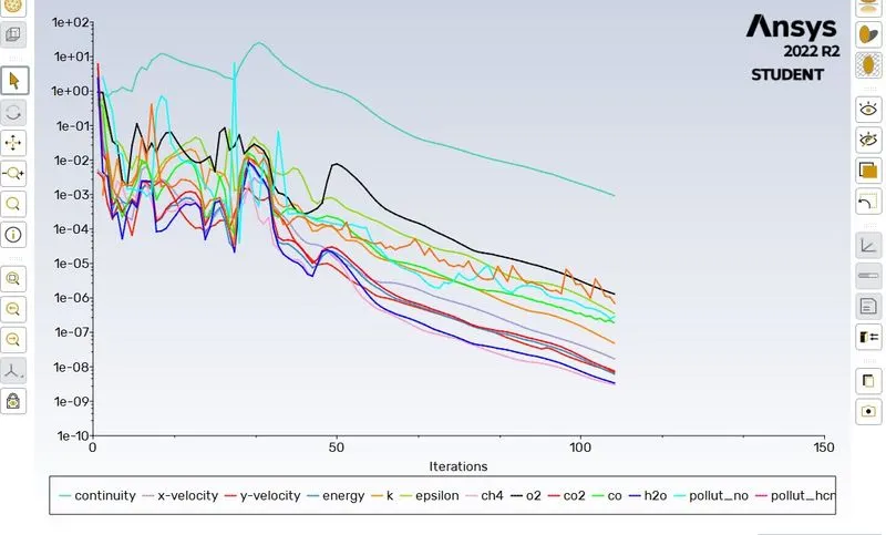
Tables and charts –

1.0%WATER-100% NATURAL GAS

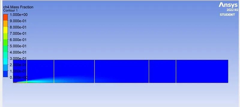
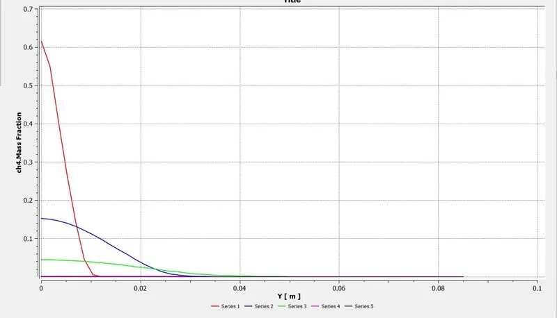
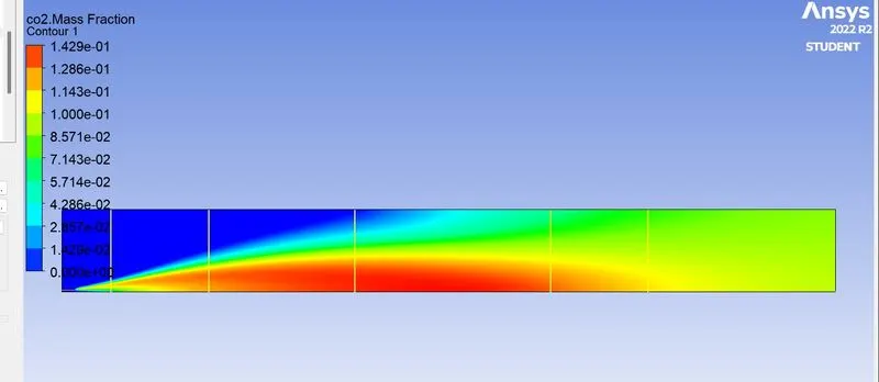
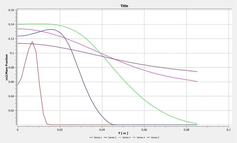
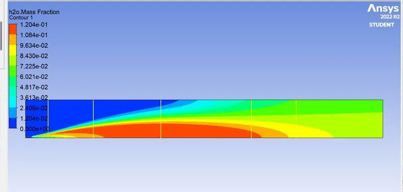
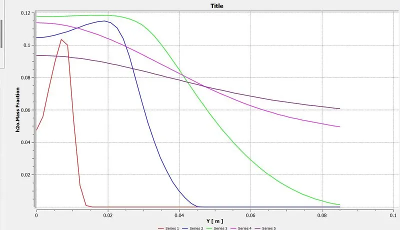
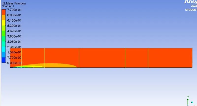
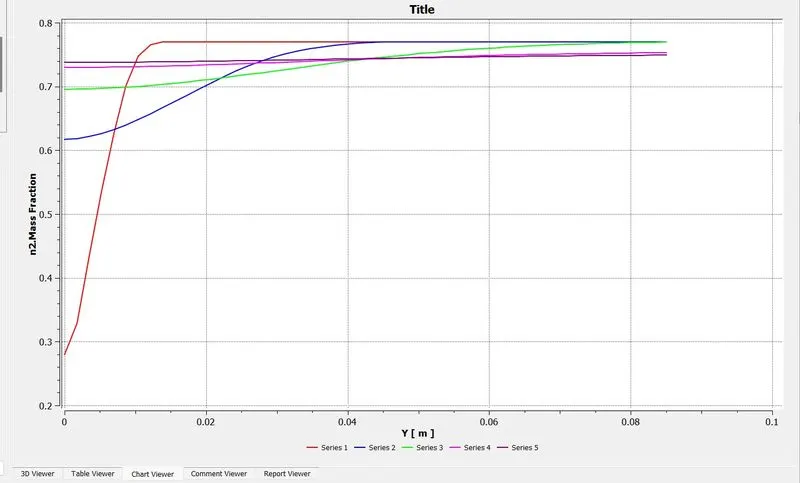
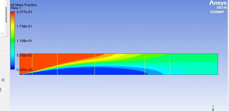
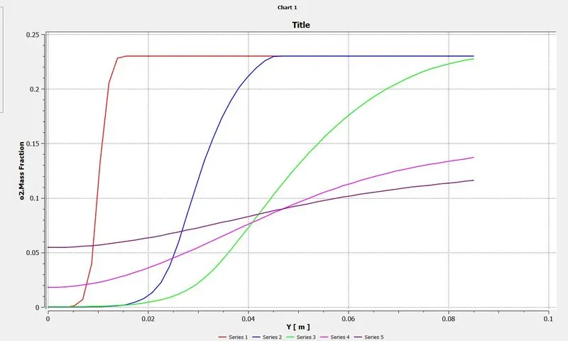
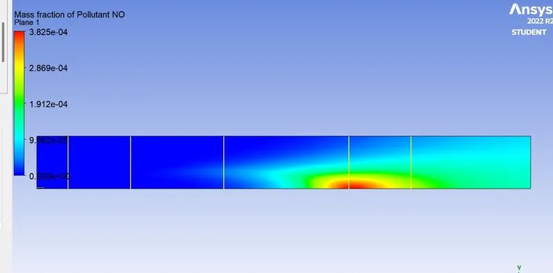
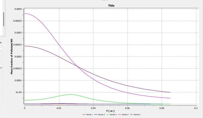
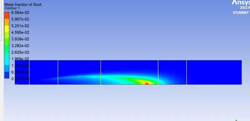
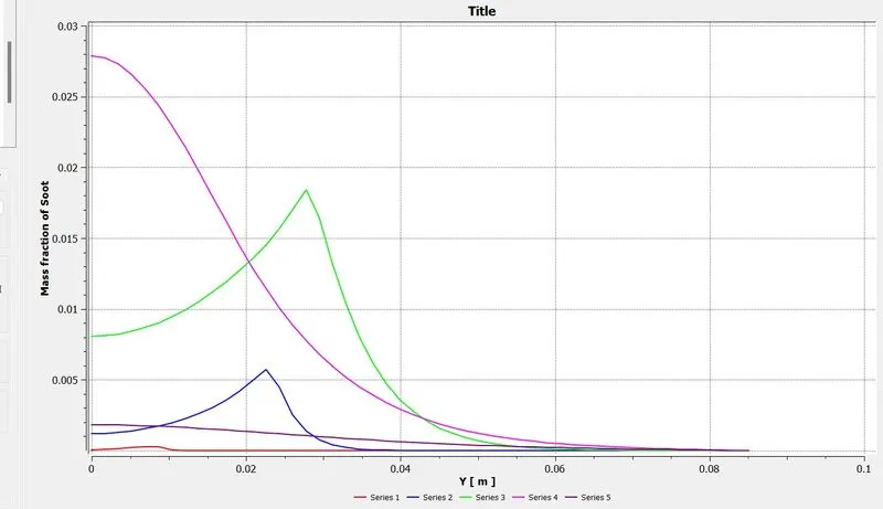
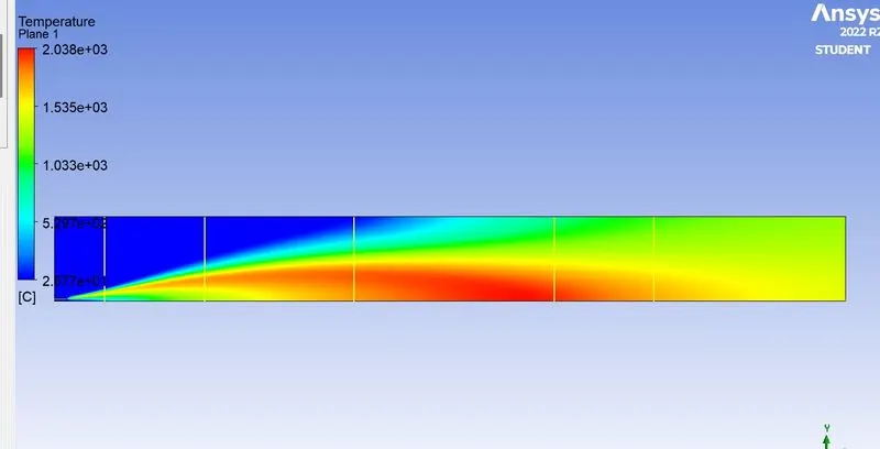
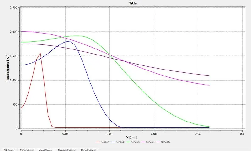
2.5%WATER-95% NATURAL GAS

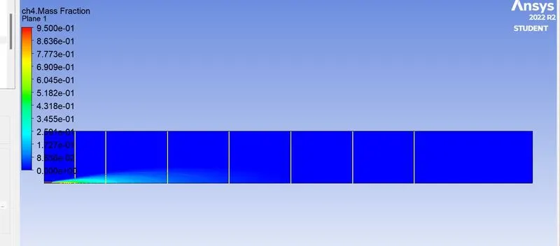
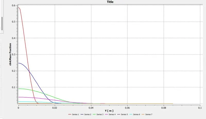
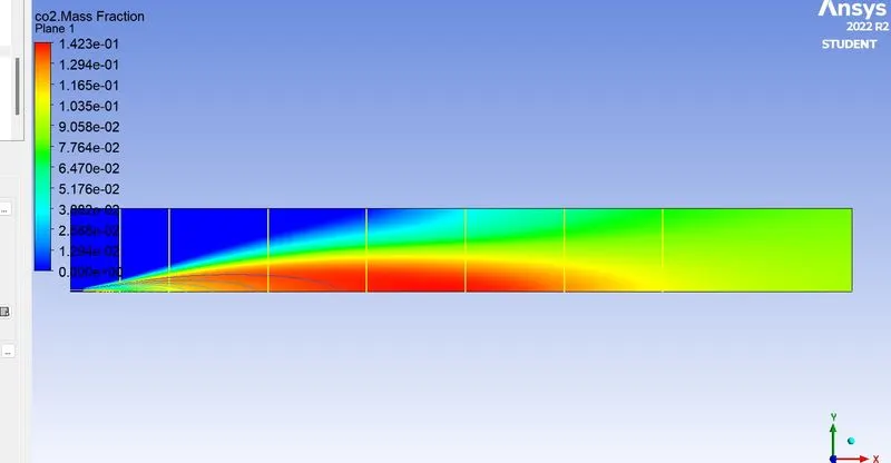
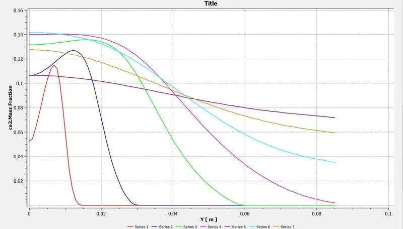
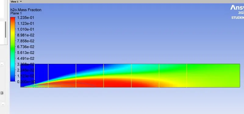
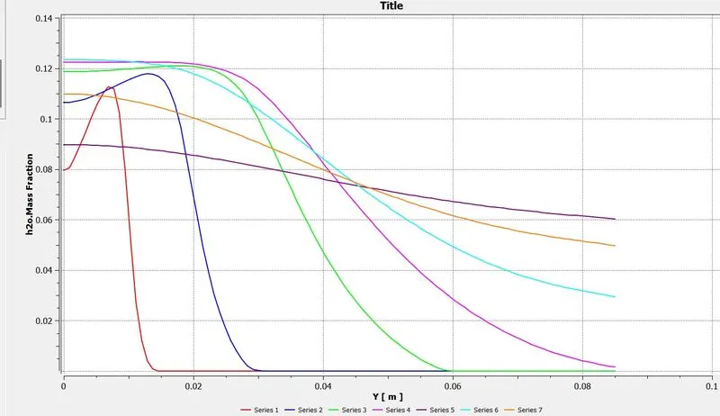
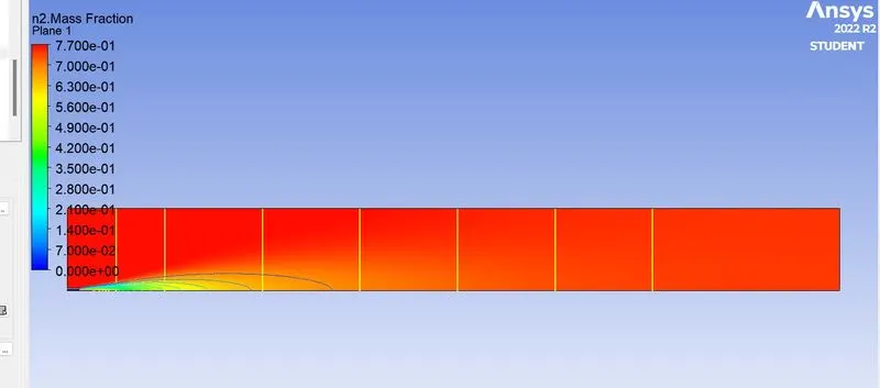
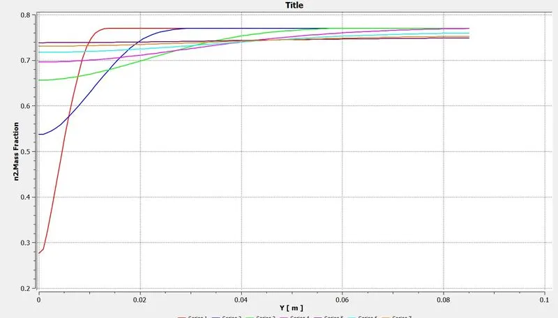
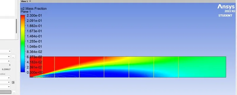
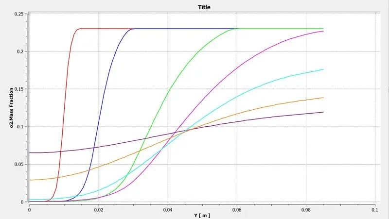
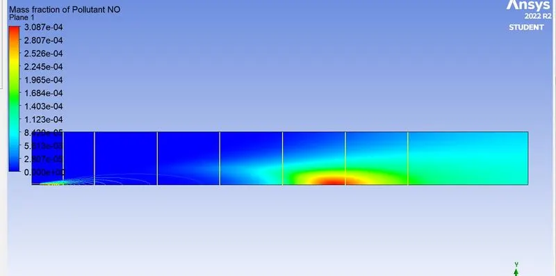
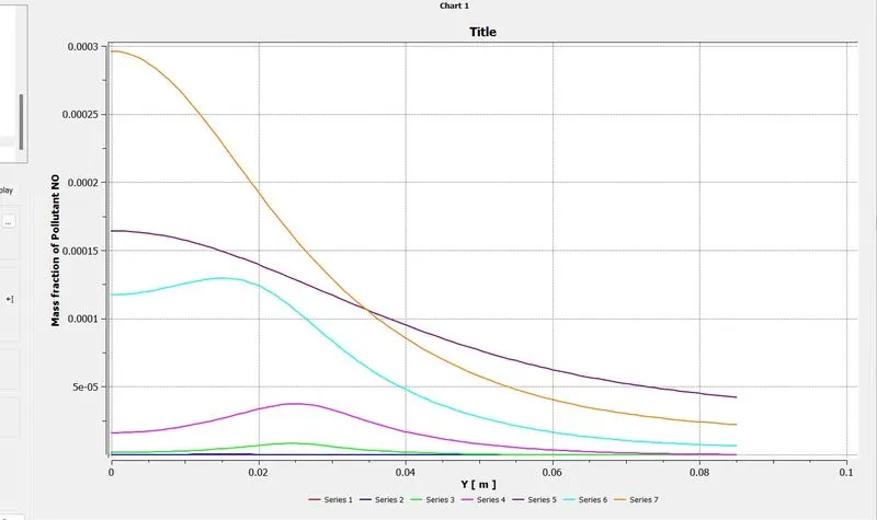
3.10%WATER-90% NATURAL GAS

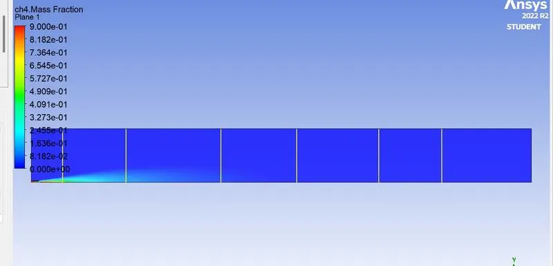
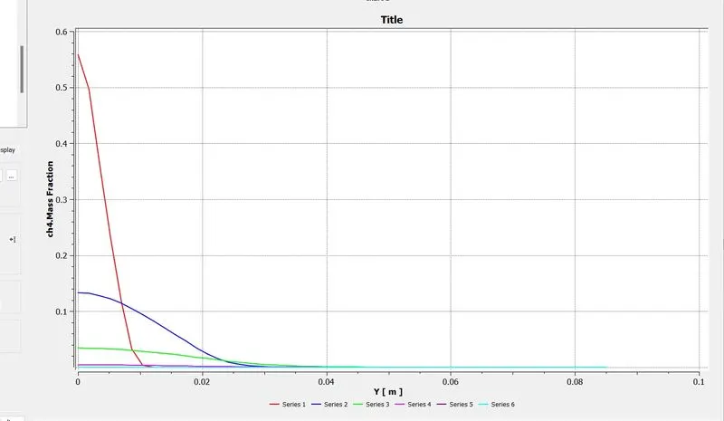
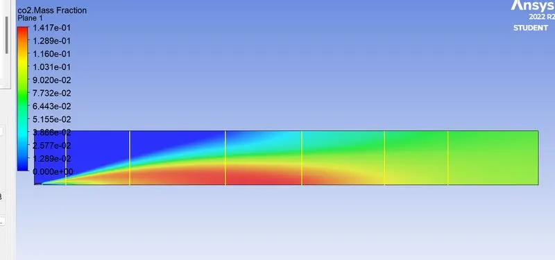
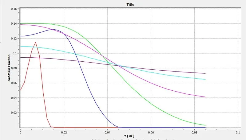
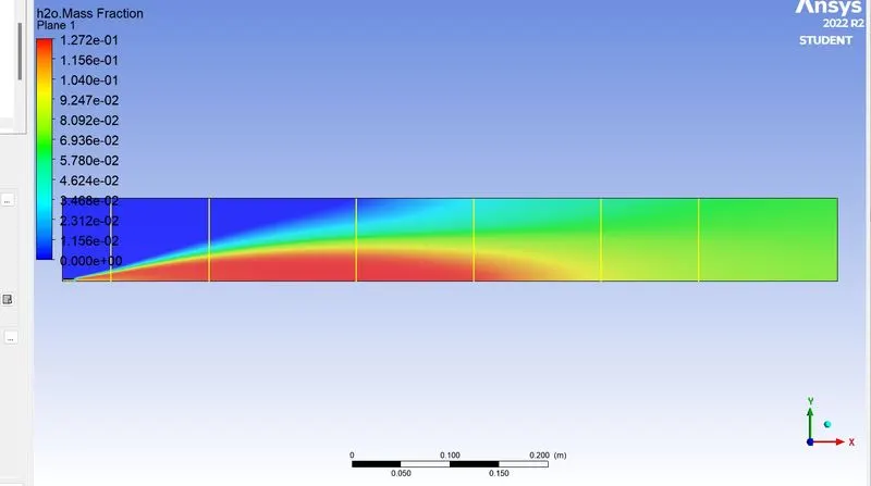
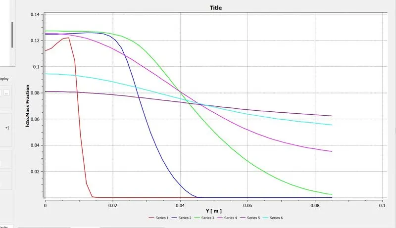
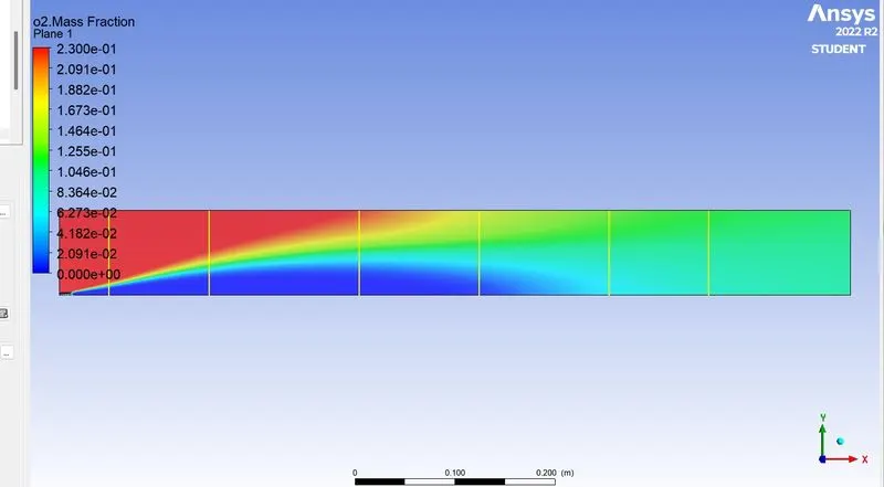
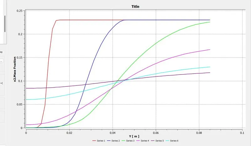
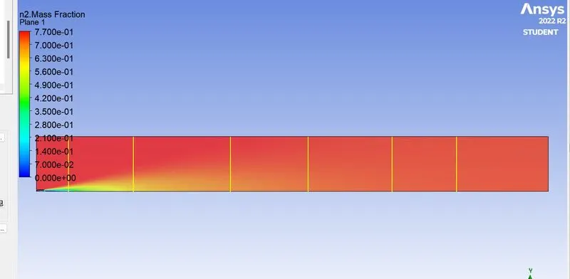
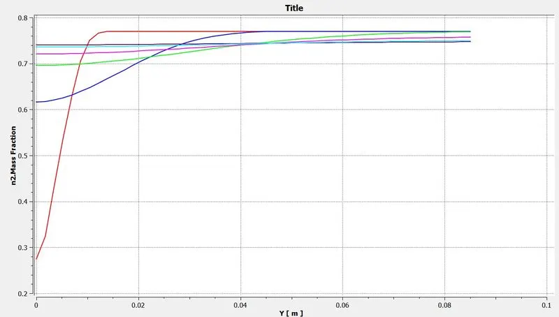
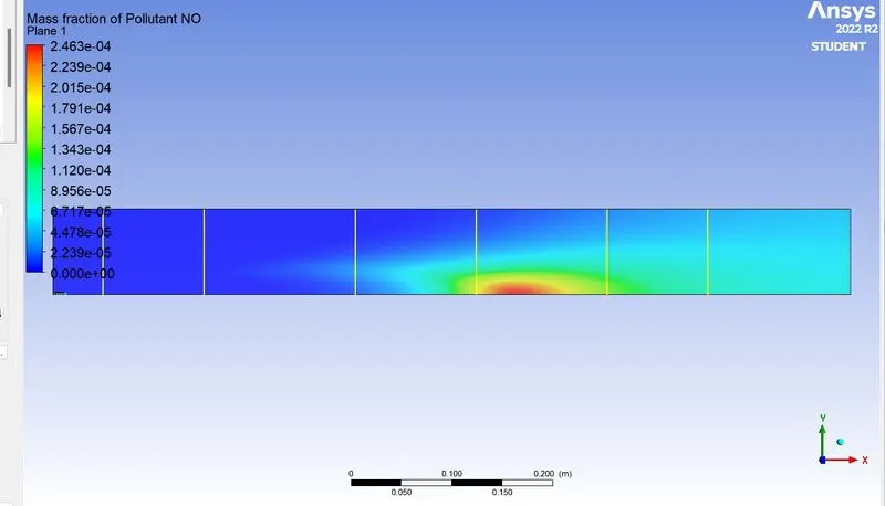
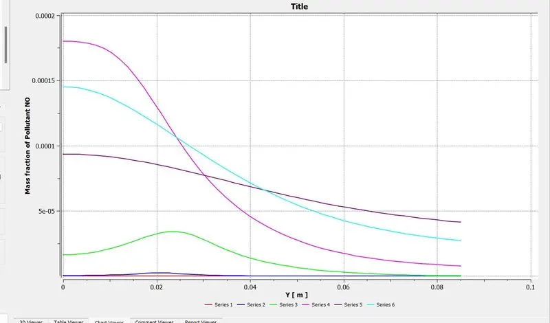
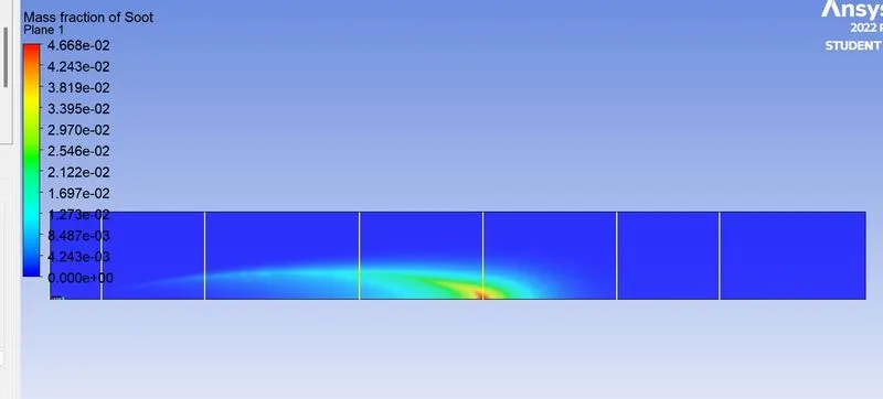
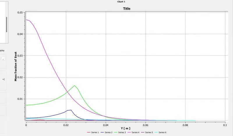
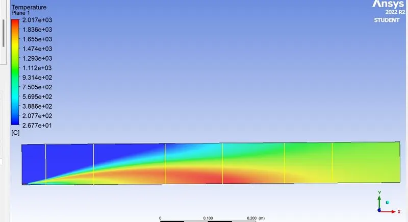
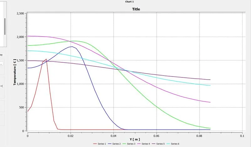
4.15%WATER-85% NATURAL GAS

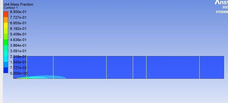
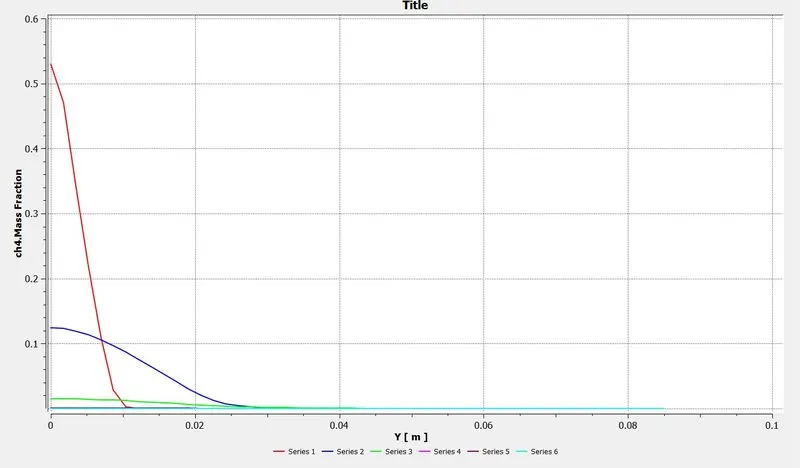
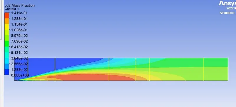
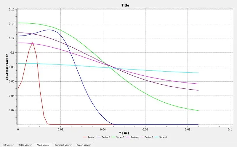
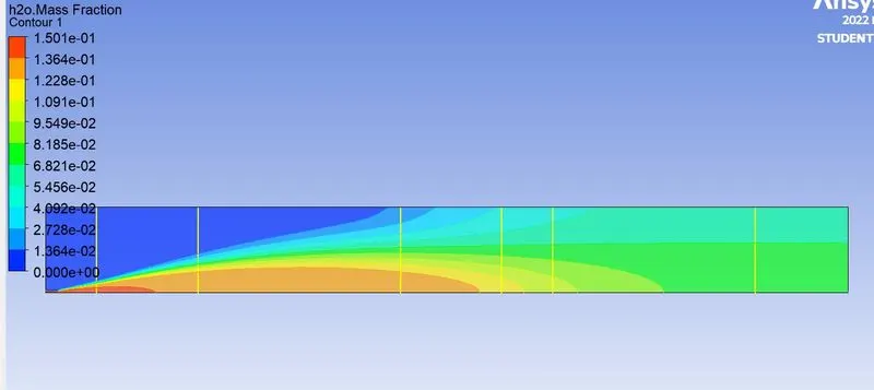
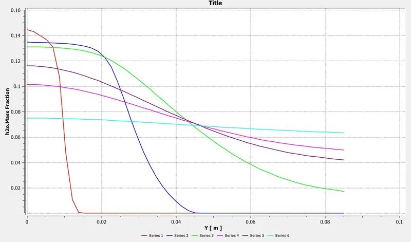
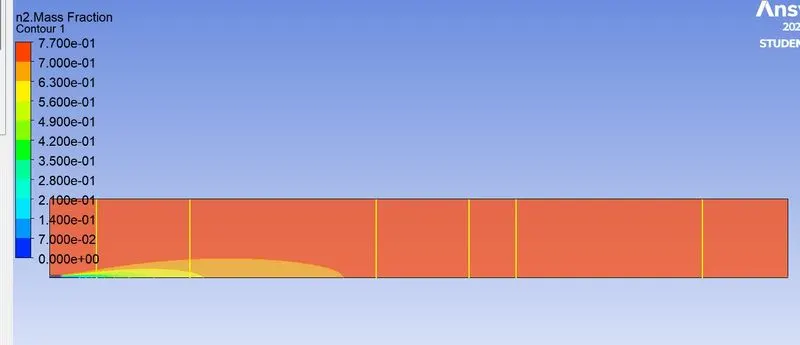
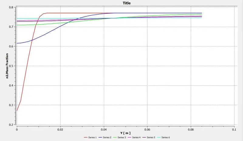
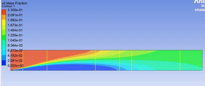
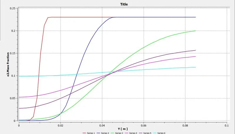
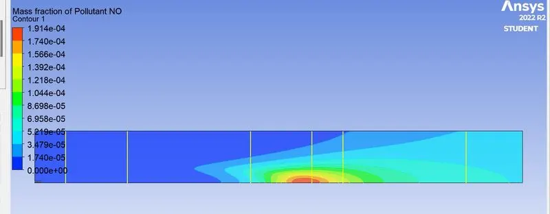
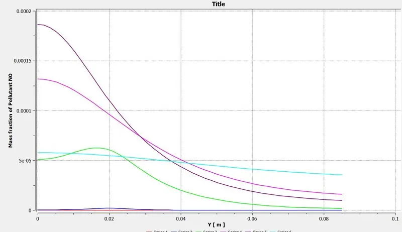
5.20%WATER-80% NATURAL GAS

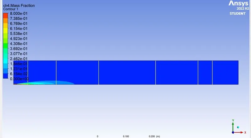
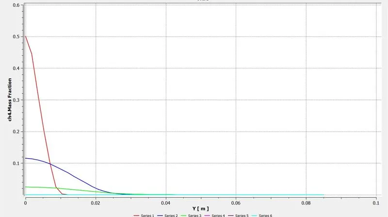
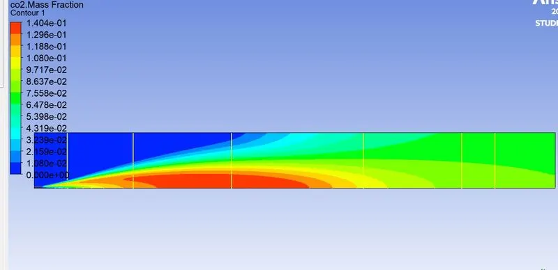
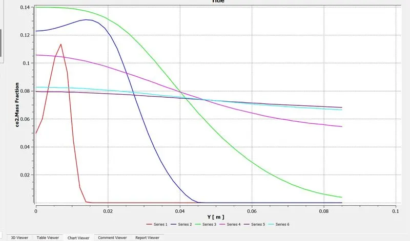
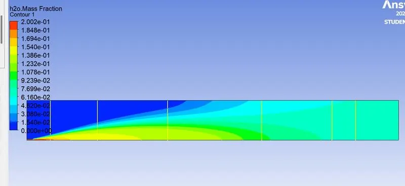
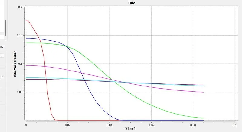
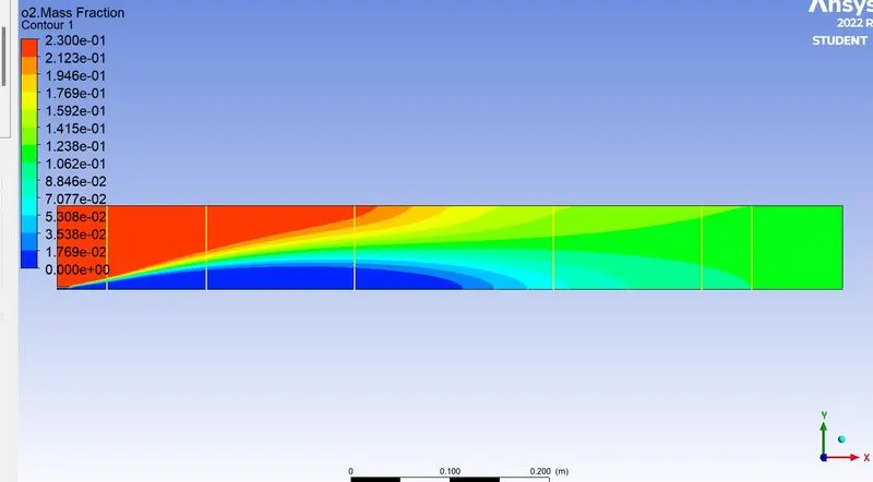
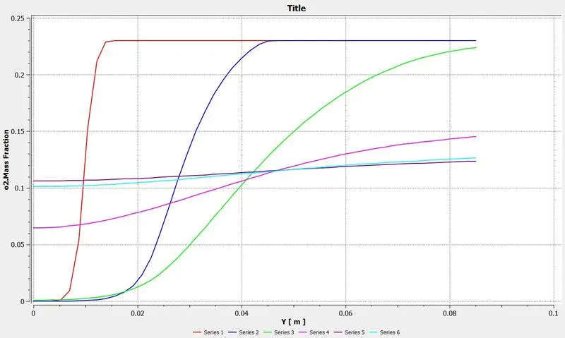
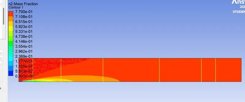
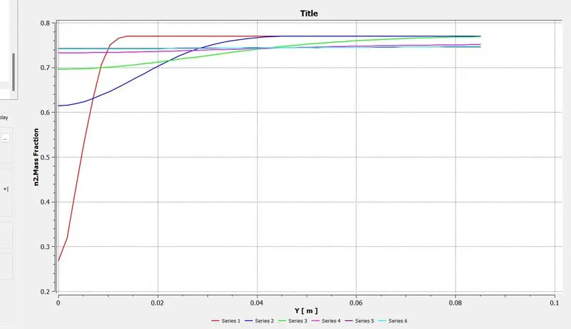
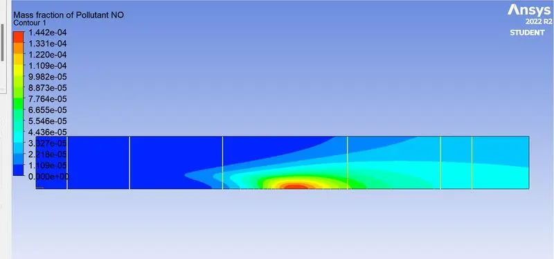
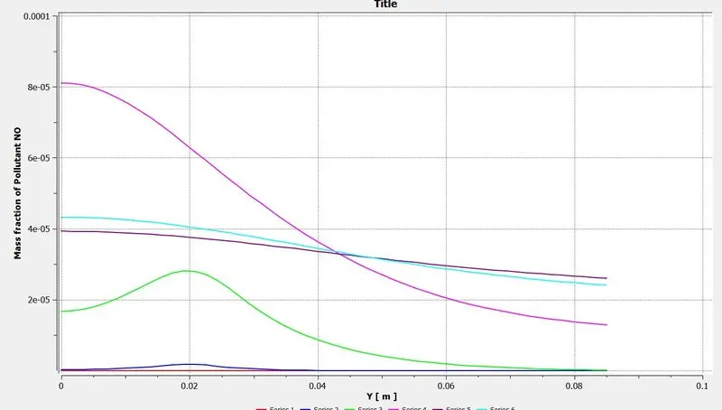
6.25%WATER-75% NATURAL GAS

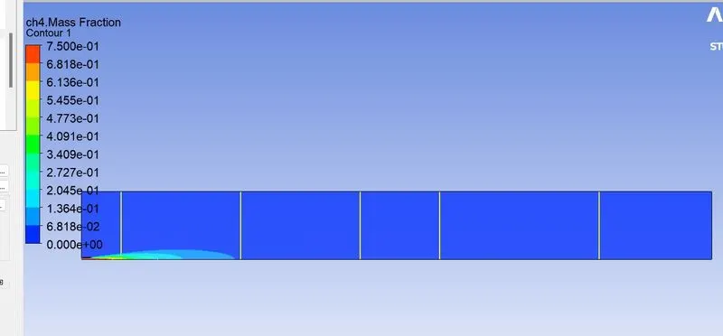
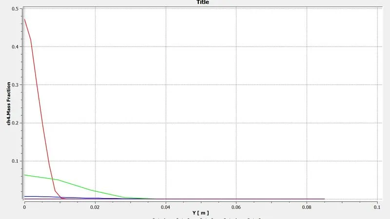
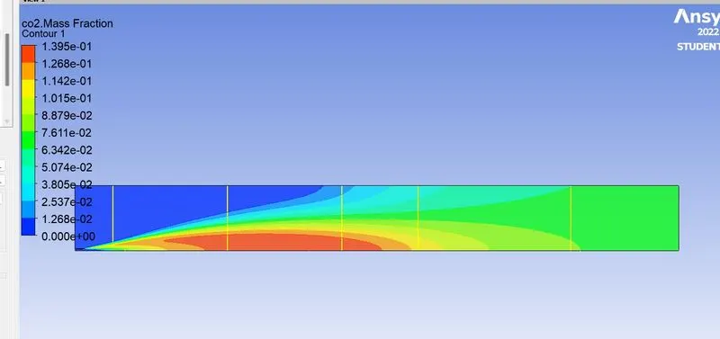
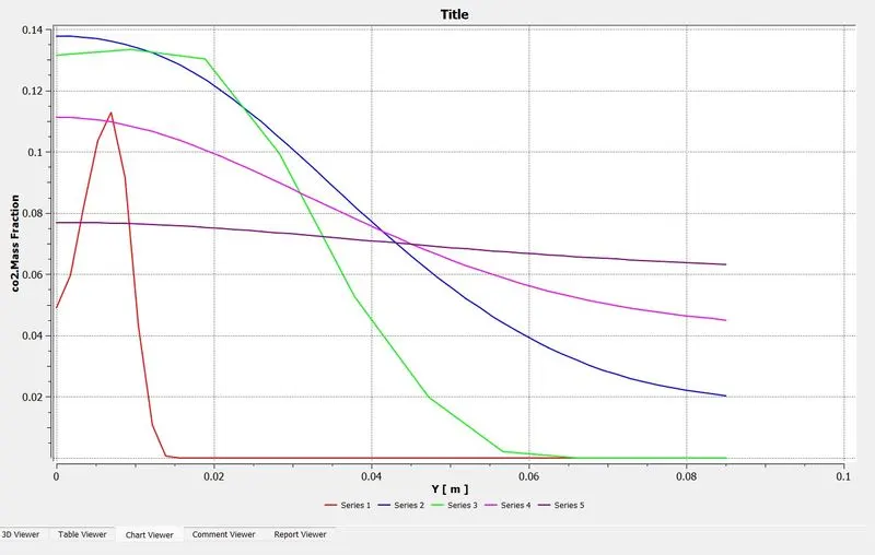
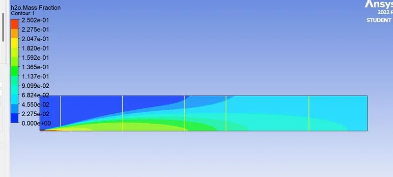
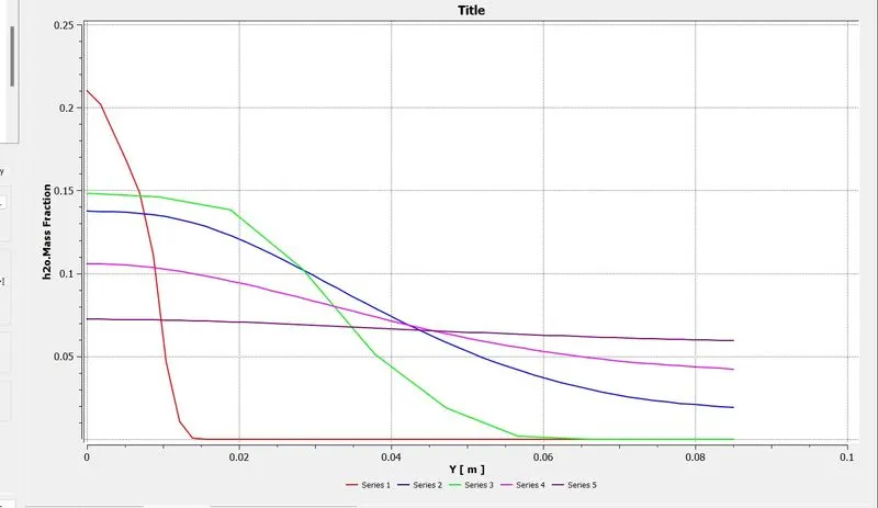
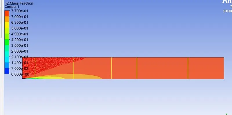
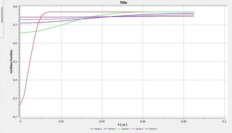
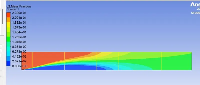
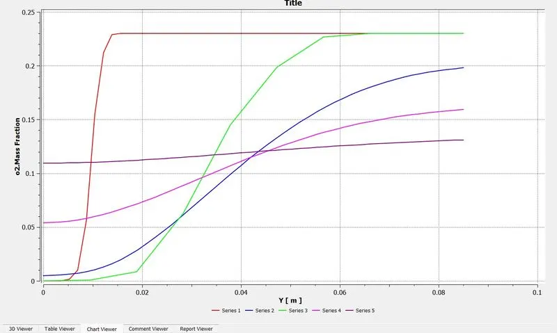
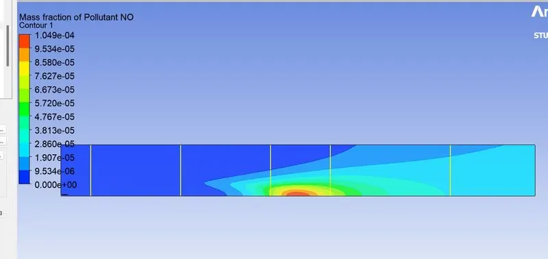
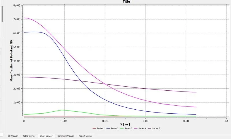
7.30%WATER-70% NATURAL GAS

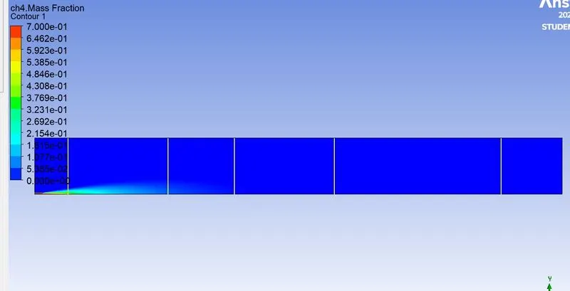
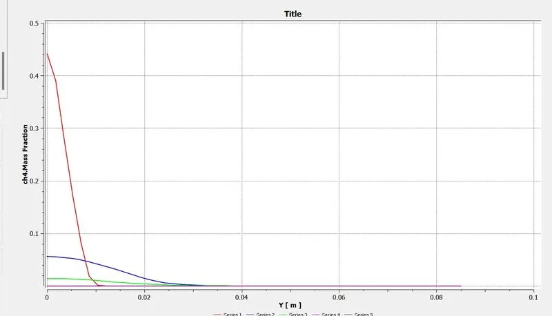
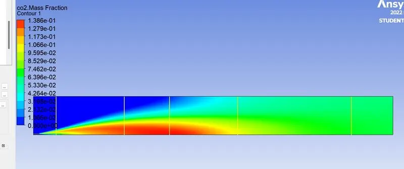
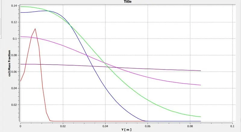
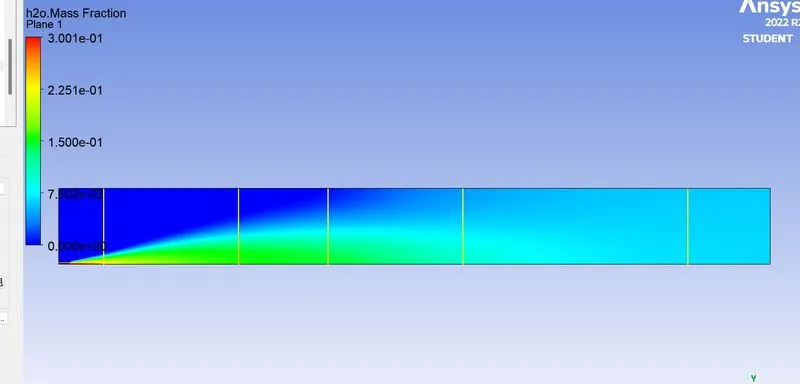
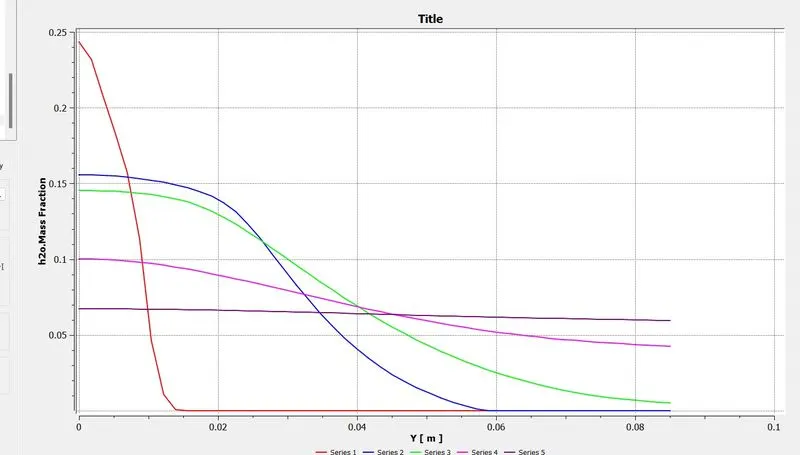
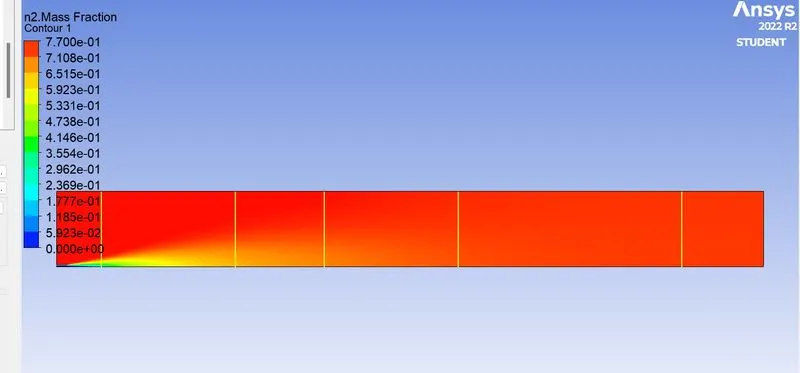
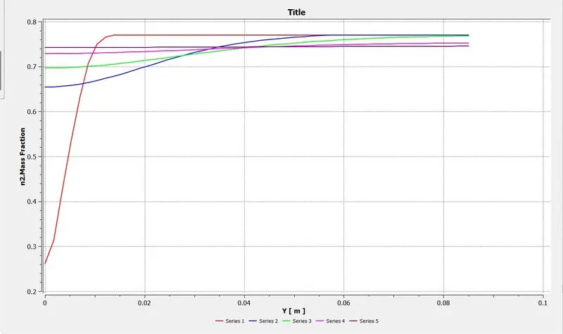
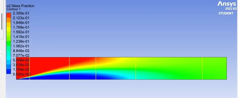
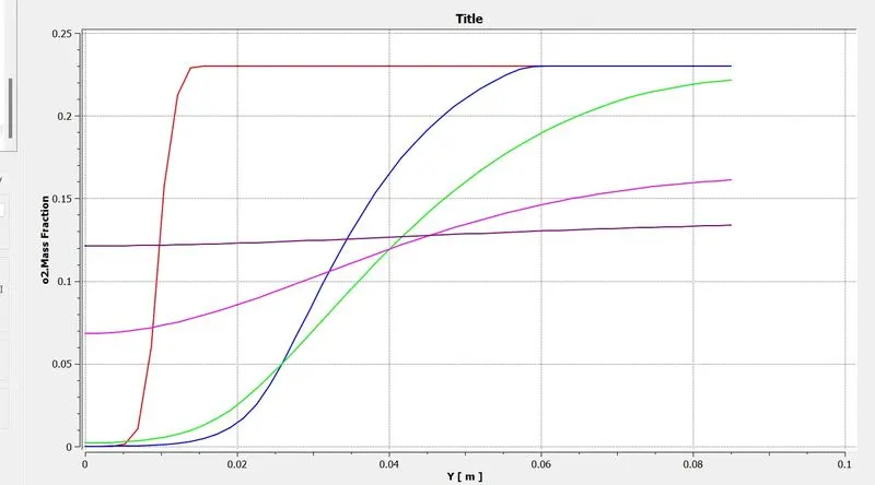
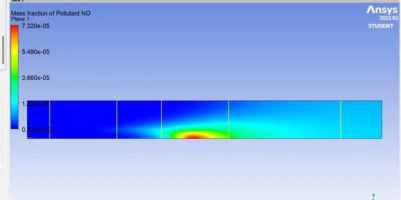
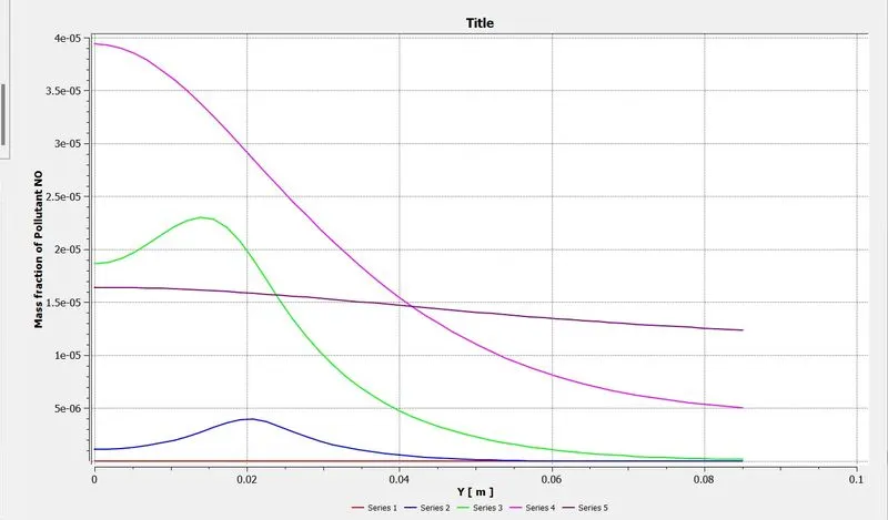
Conclusions and inferences –

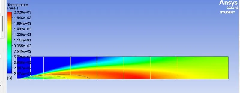
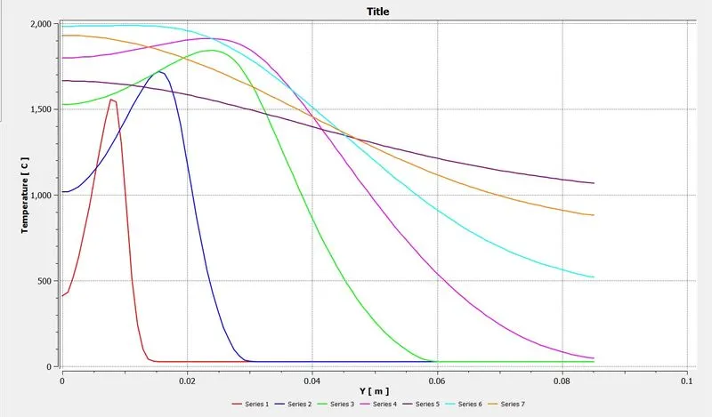
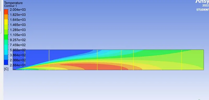
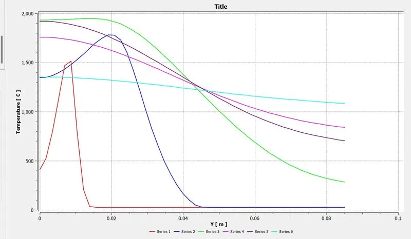
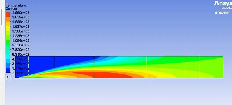
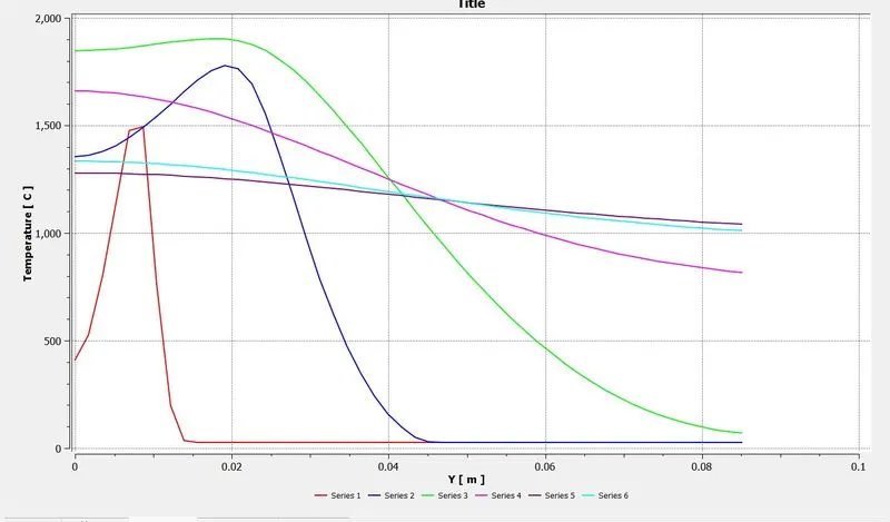
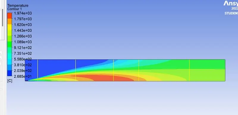
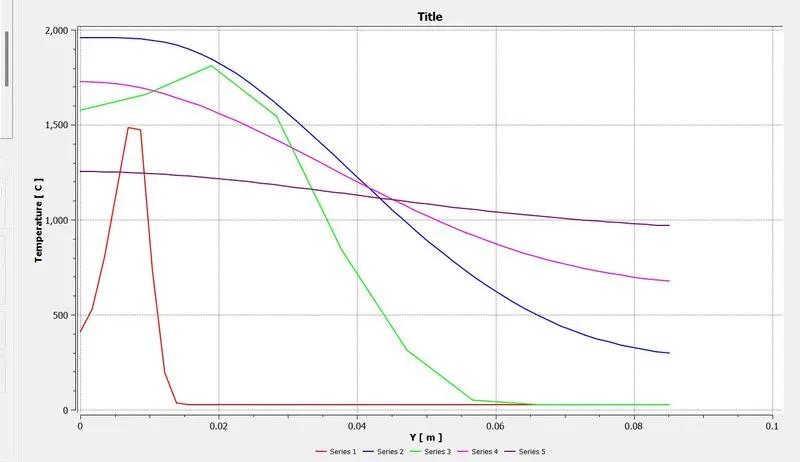
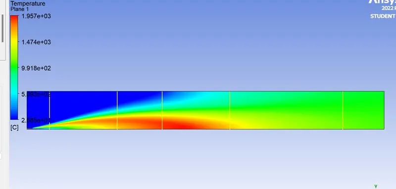
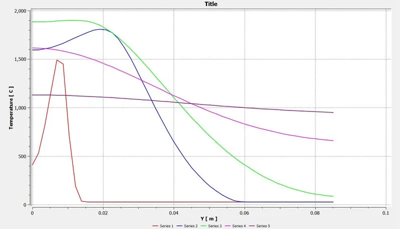
1. Maximum Temperature at outlet – As the water content in the fuel is increased, the average temperature decreases thus indicating that water aids in cooling the entire system
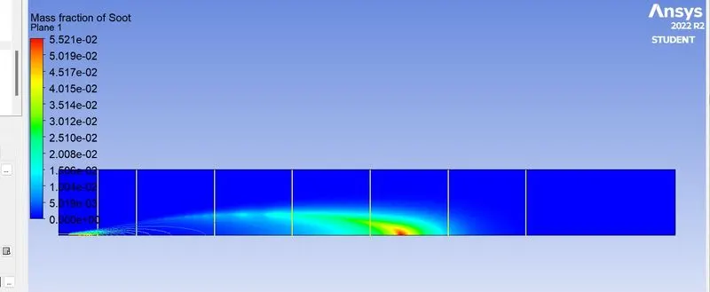
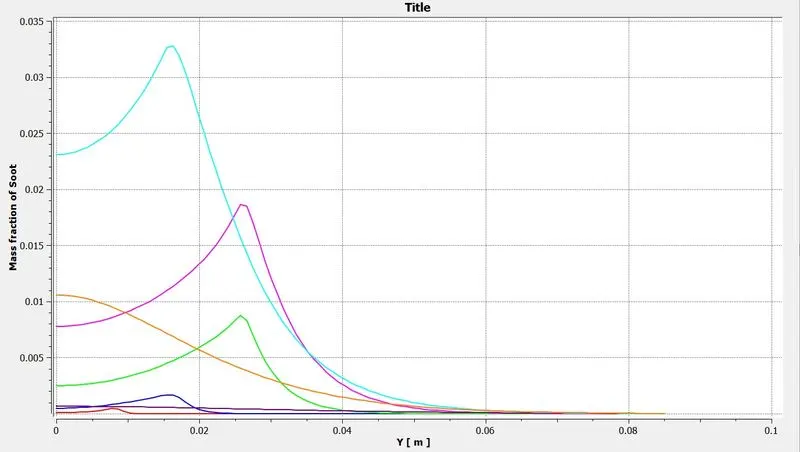
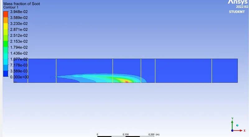
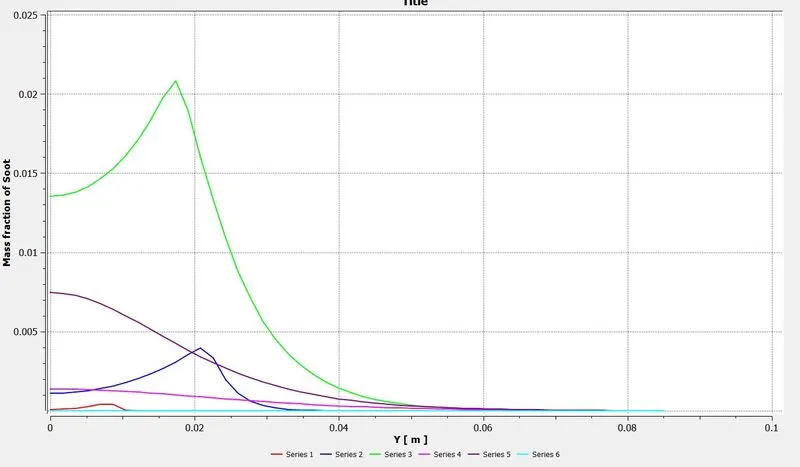
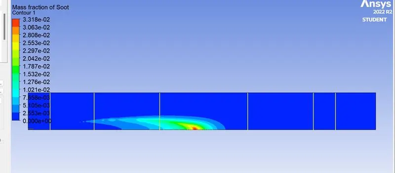
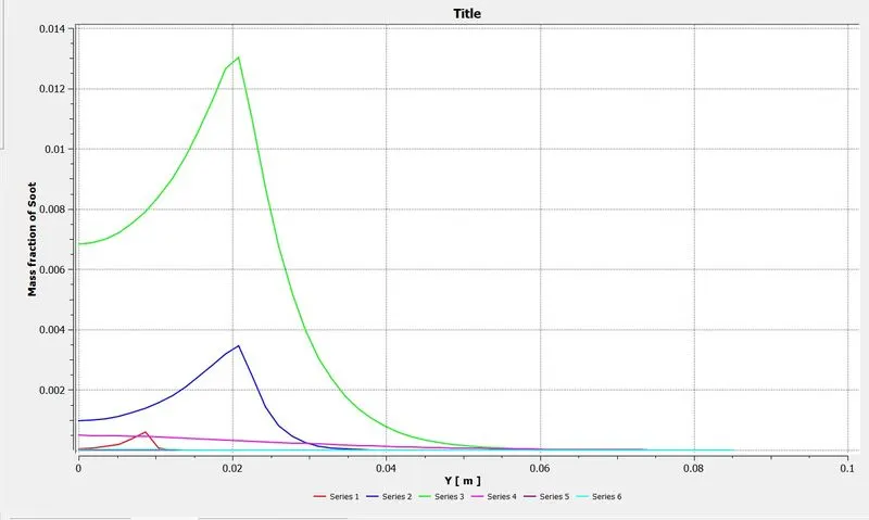
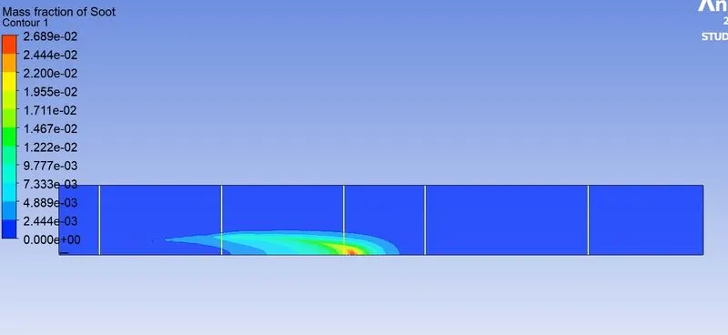
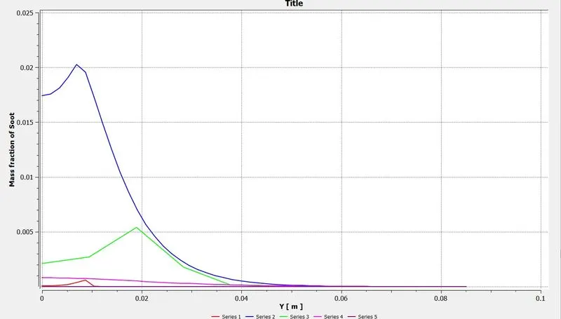
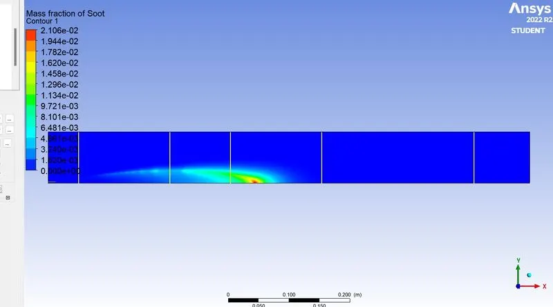
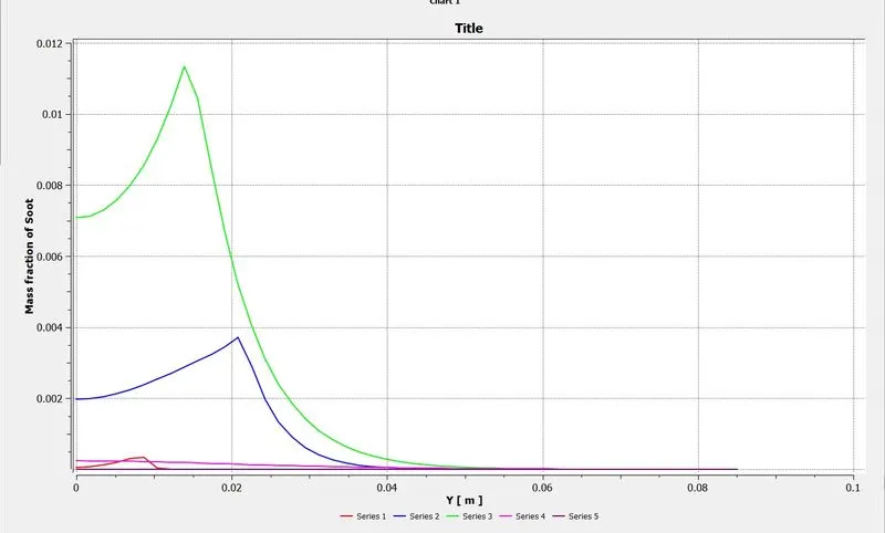
2. SOOT emissions – The SOOT emissions decrease drastically after the addition of water. This can be understood by the 2 iterations – 0% water and 5% water. In the 5% water iteration, the contours are completely blue showing almost 0 mass fraction of Soot. However, as we increase the water content, the contours show slight amount of soot near the outlet
3. NOx emissions – As the water content increases from 5% to 30% the NOx emissions are also decreasing.