Week 10 - Simulating Combustion of Natural Gas.

SIMULATION OF NATURAL GAS COMBUSTION

Introduction:

Methane is a main component of biogas an fossil natural gas and also stands at a transition point of fossil fuel and bio fuel. It is also known for its lesser harmful pollutants compared to other gaseous or liquid fossil fuels, and hence an environment-friendly fuel. It is widely used in combustion research due its relatively small fuel molecule and simpler chemical kinetics. Prediction of methane performance over a wide range of conditions with respect to temperature, pressure and equivalence ratio is fairly simple. Explicit chemistry is needed to study methane combustion in real-time industrial CFD applications. Due to limitations of computing capacity, modelling has been performed with simplified chemical descriptions like global chemistry and flamelet approach. however these do not resolve the interaction between chemistry and turbulence on smallest scales. they are also not used for characterization of pollutant formation.

Large eddy simulations are suitable for modelling of turbulent combustion coupled with chemical kinetics. but due to computational costs, detailed kinetics schemes are not feasible. With current capacity, 80-100 reactions represent an upper limit in terms of mechanism size. It has been shown that this number of species is adequate to model important combustion characteristics of common hydrocarbon fuels.

Chemical kinetics of combustion:

Methane is an important fuel for gas turbine and gas engine combustion, and the most common fuel in fundamental combustion studies. For flame simulations, a reduced mechanism with only 42 irreversible reactions gives a good agreement with the experimental data. For combustible mixtures with the addition of hydrogen, carbon dioxide, and water the results can be seen as comfortably accurate compared to pure methane-air mixtures.

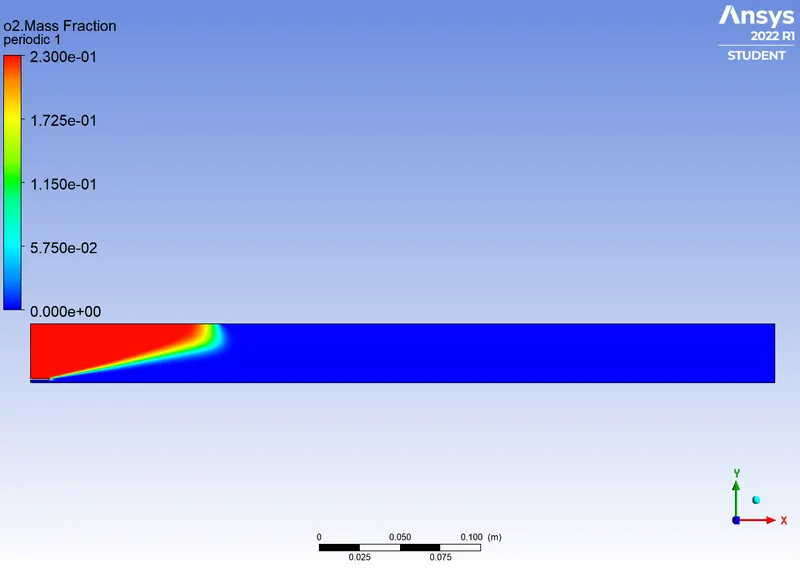
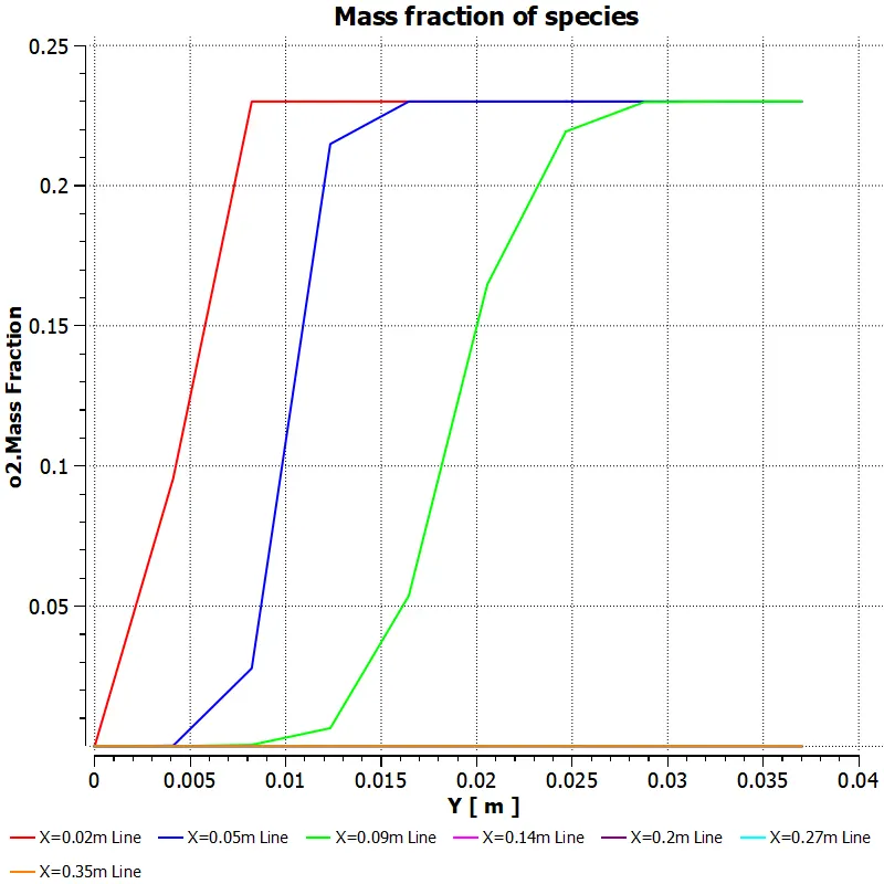
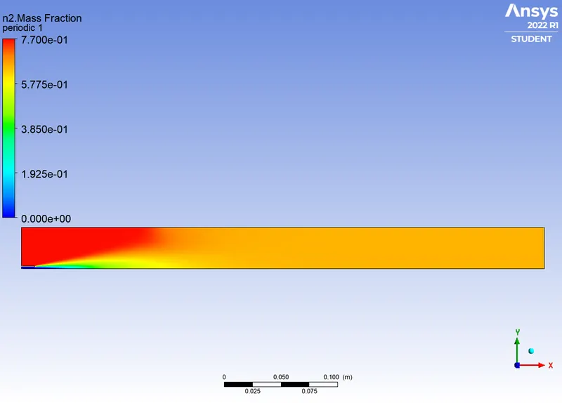
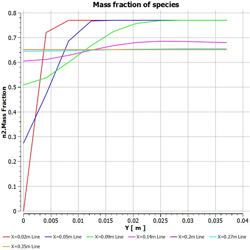
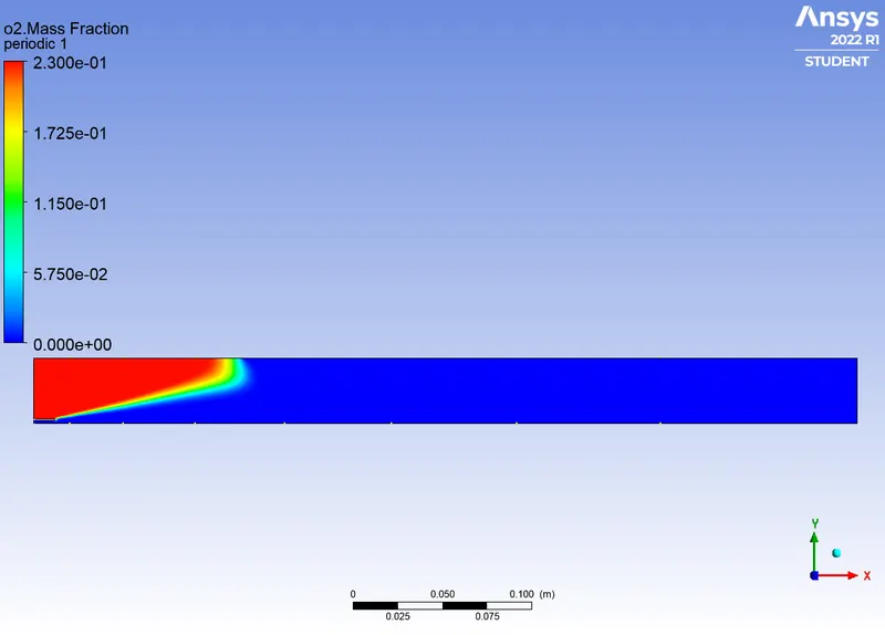
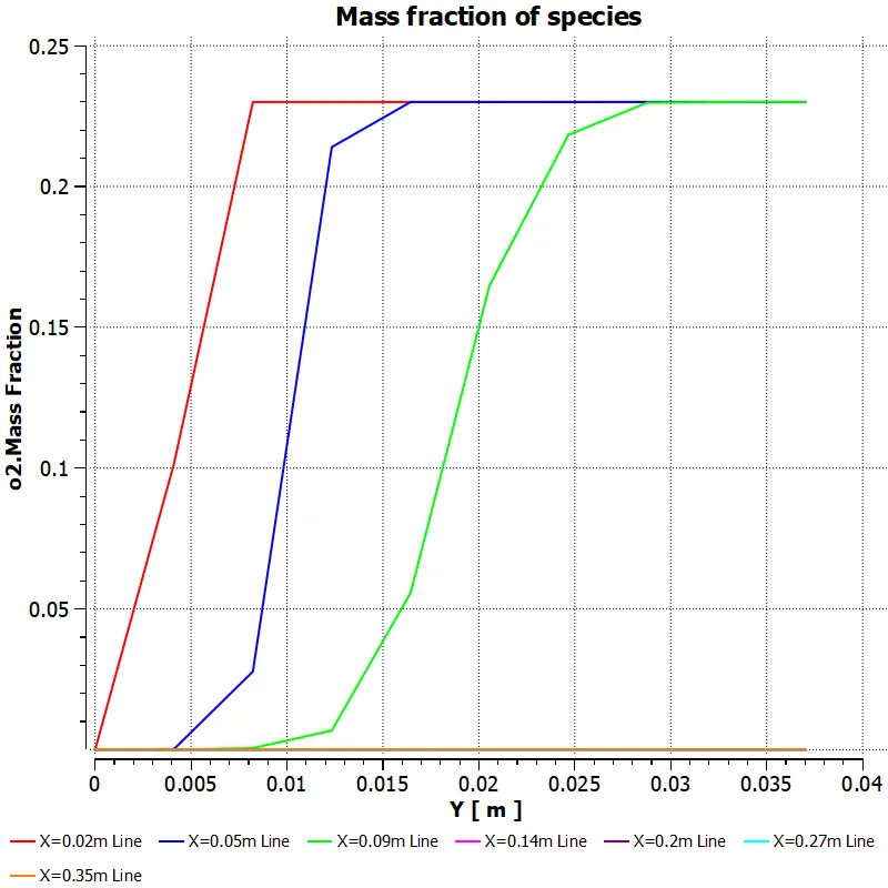
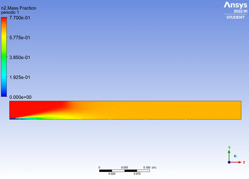
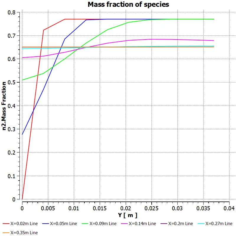
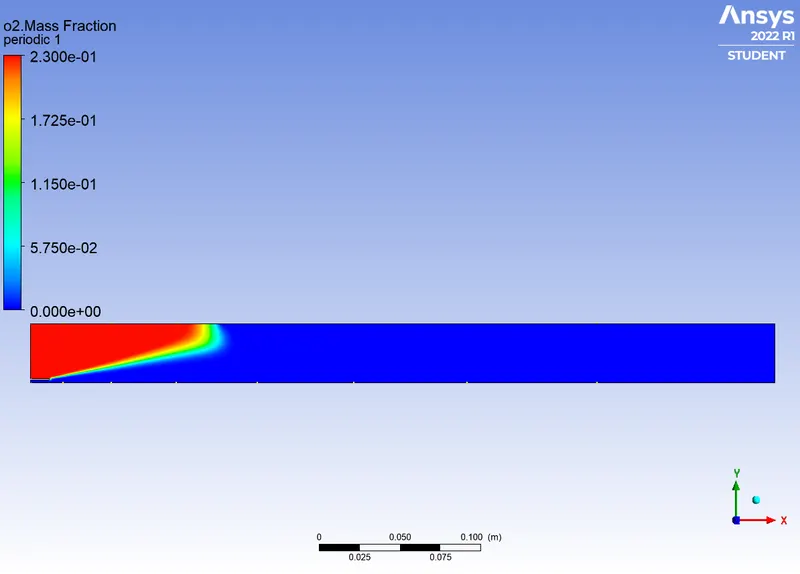
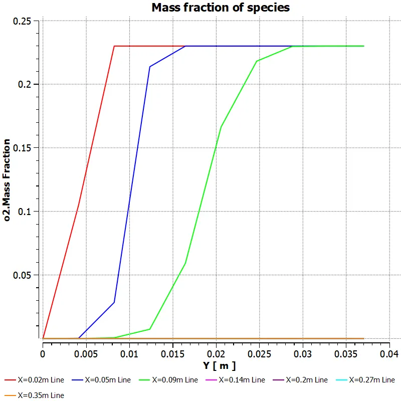
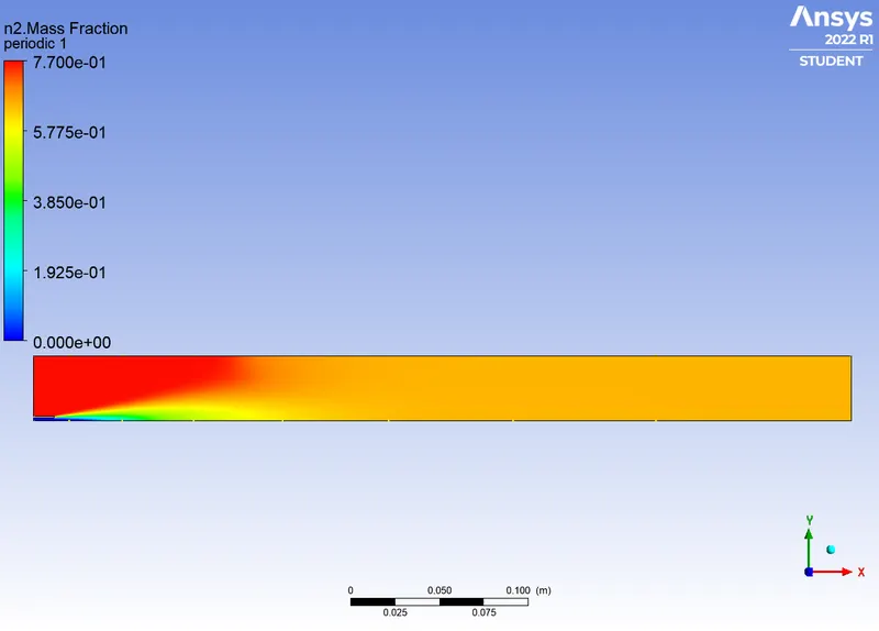
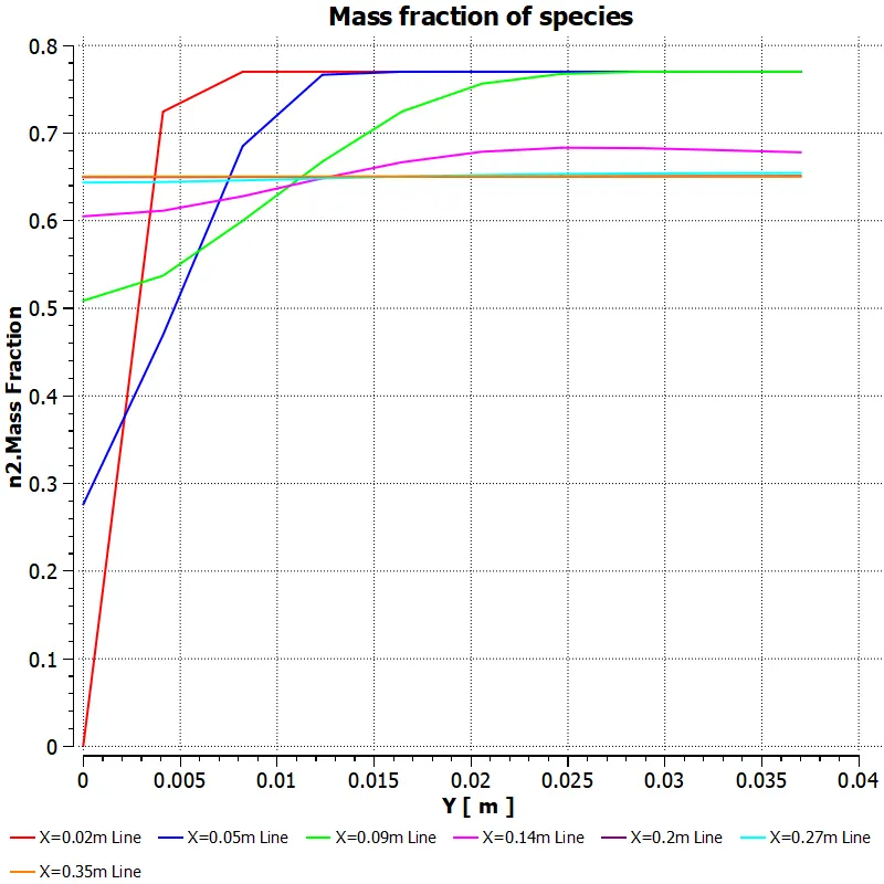
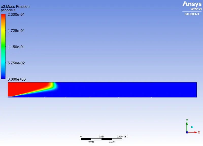
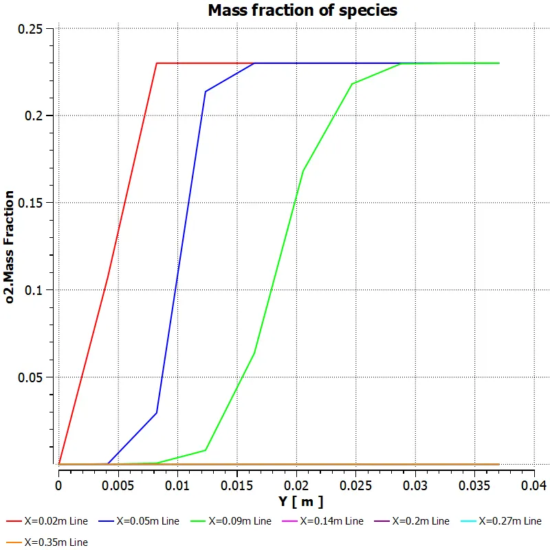
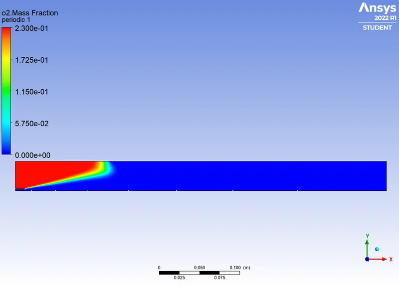
The chemical reaction for methane fuel combustion is: CH4 + ar(O2 + 3.76N2) = aCO2 + bH2O + cN2, where a,ar, b,c are variables to calculate the quantity of the species. Balancing the equation gives 2 moles of O2 and 7.52 moles of N2, converting this to mass fraction terms, for 1 CH4 there are 0.23 O2 and 0.77 N2.

Species transport model - Eddy dissipation model:

Species transport model based on species transport equation is selected to model the chemical reactions in a composition of various species like CO, CO2, N1, H2 and CH4. These reactions are solved by the conservation equations relating to convection, diffusion of each species. The net rate of production of species relation with the diffusion flux of species and concentration gradients for a turbulent flow is analysed by this method. The rate of the chemical reaction is computed using an expression that accounts for the temperature and pressure by ignoring the effects of turbulent eddies.

Eddy dissipation model provides an empirical expression for the mean reaction rate based on the assumption that chemical reaction occurs in the regions where the turbulence energy takes place. It uses the rate of dissipation of eddies containing reactants and products to determine the reaction rates. In the purest form, it computes reaction rates based on rates of turbulent mixing. An implicit assumption is that the chemical kinetic rates are considerably faster than rates of turbulent mixing, that is the rate-limiting process. An important aspect in using Eddy dissipation model is that it is prone to the problem of spurious ignition, which is the phenomenon of ignition of unburnt mixture at regions far ahead of flame. Estimation of rate of reaction based on mixing time scales is also called as Eddy dissipation model. Modified for of Eddy dissipation model takes account of the dependence of the mean reaction rate on the ratio of the turbulent kinetic energy.

Run cases:

For this simulation, the cases are split into 7 cases across two parts. The 1st part being done with a pure methane fuel and the 2nd part is done on 6 cases of methane fuel with H2O inclusions. The percentage of inclusions in part 2 fuel is varied among 6 ranges.

Part 1 (Case 1): Pure CH4 fuel combustion

Air velocity = 0.5m/s

Air inlet - Oxygen fraction percent = 0.23

Air inlet temperature: 300K

Fuel velocity = 80m/s

Fuel inlet - CH4 fraction percent = 1

Fuel inlet temperature: 300K

Part 2: CH4 fuel with H2O inclusions

Air velocity = 0.5m/s

Air inlet - Oxygen fraction percent = 0.23

Air inlet temperature: 300K

Fuel velocity = 80m/s

Fuel inlet temperature: 300K

Case 2.1	Case 2.2	Case 2.3	Case 2.4	Case 2.5	Case 2.6
CH4 level: 95% H2O level: 5%	CH4 level: 90% H2O level: 10%	CH4 level: 85% H2O level: 15%	CH4 level: 80% H2O level: 20%	CH4 level: 75% H2O level: 25%	CH4 level: 70% H2O level: 30%

Procedure:

Step 1:Geometry

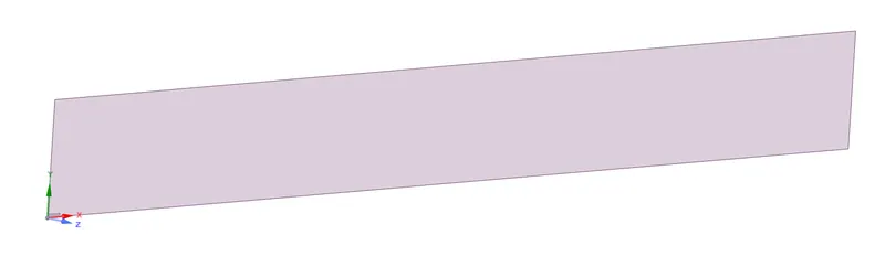
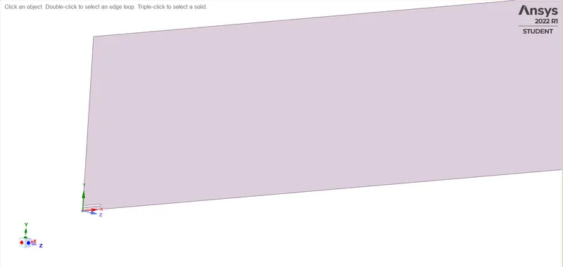
The given geometry of the combustor is imported in the Space Claim component. It is the 3D model of a Cylindrical combustor with a fuel inlet. Due to computational capacity, this geometry has to be converted into a 2D axisymmetric geometry.

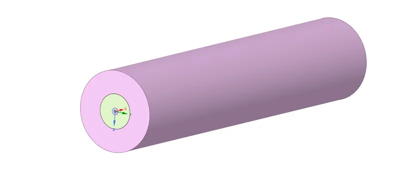
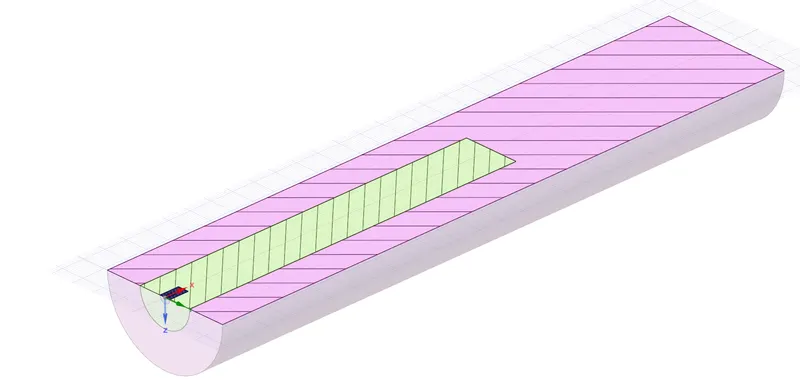
Three axes at the origin are created for splitting the body. Split body command is used to split the body into a quadrant to obtain an axisymmetric geometry.

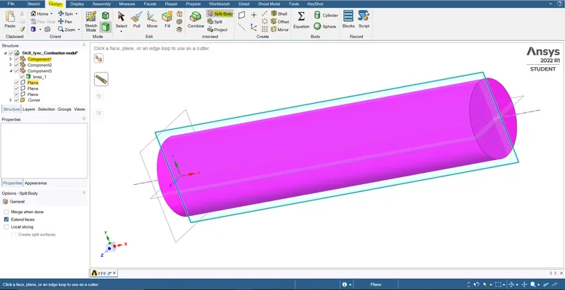
The split body command is executed in XY axis and XZ axis o obtain a quadrant.

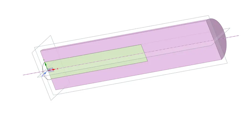
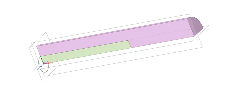
The faces at the X-Y axis is copied and pasted in a new design document and saved.

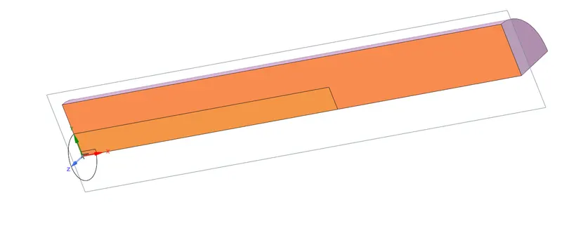
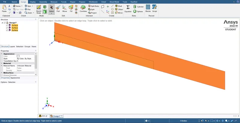
The new surface geometry is checked for shared topologies and the extra edges are removed.

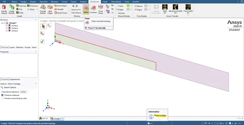
The final geometry obtained as a single surface is the required geometry and is exported to the meshing component.

Step 2:Meshing

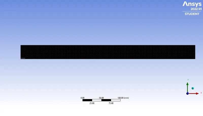
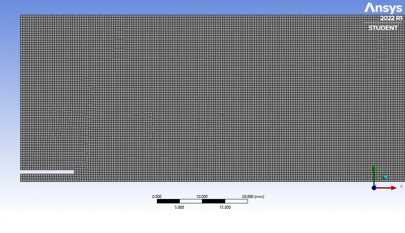
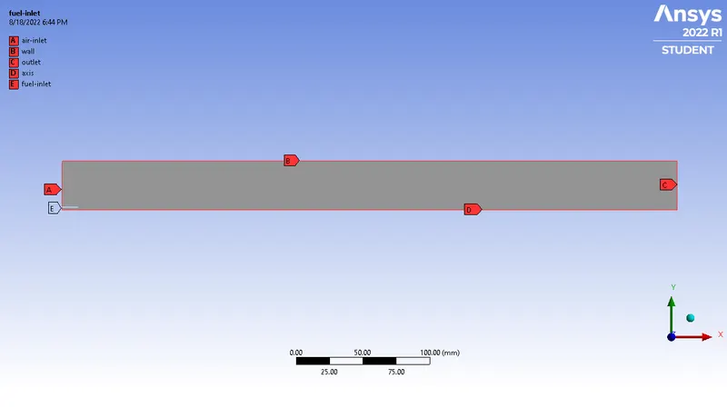
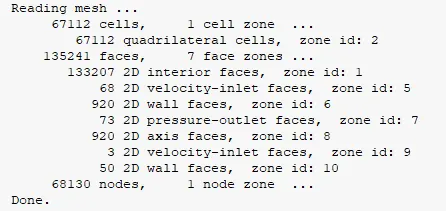
The default method is selected for meshing and the element size is maintained at 0.5mm for a convenient simulation. The air inlet, fuel inlet and outlet are named by selecting. The upper wall is named as wall after its boundary condition. The lower wall is named as axis. The proximity gap factor is set at 3 cells.

Step 3: Solver setup

3.1: Basic Solver setup

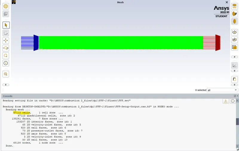
The basic solver settings are updated after checking the mesh and boundary names are updated.

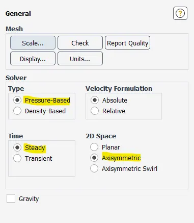
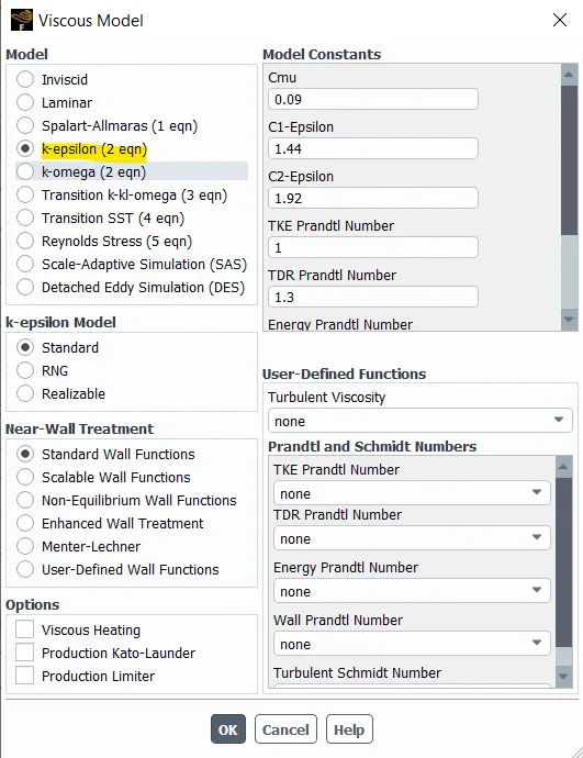
K-Epsilon model is selected with the geometry assigned as 2D axisymmetric.

3.2: Species Transport combustion model setup

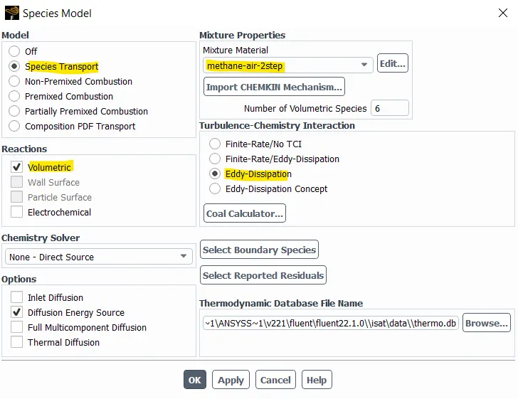
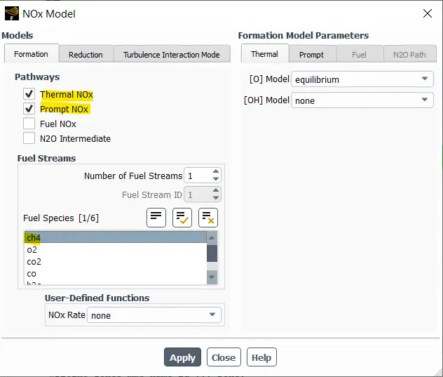
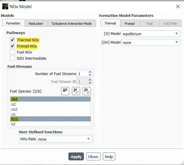
The Species transport model is modified for the current case. Methane-air 2 step mixture is selected and volumetric reactions. Eddy dissipation model is selected. The NOx and Soot model is also modified with CH4 fuel and O2 oxidant.

For Part 1 pure methane fuel , the soot model is updated with CH4 as the only fuel.

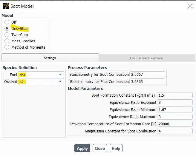
For part 2 fuel with inclusions, CH4 and H2O are updated as the fuels in the soot model.

3.3: Input and output parameters for part 2 setup

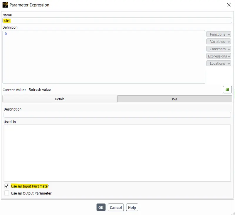
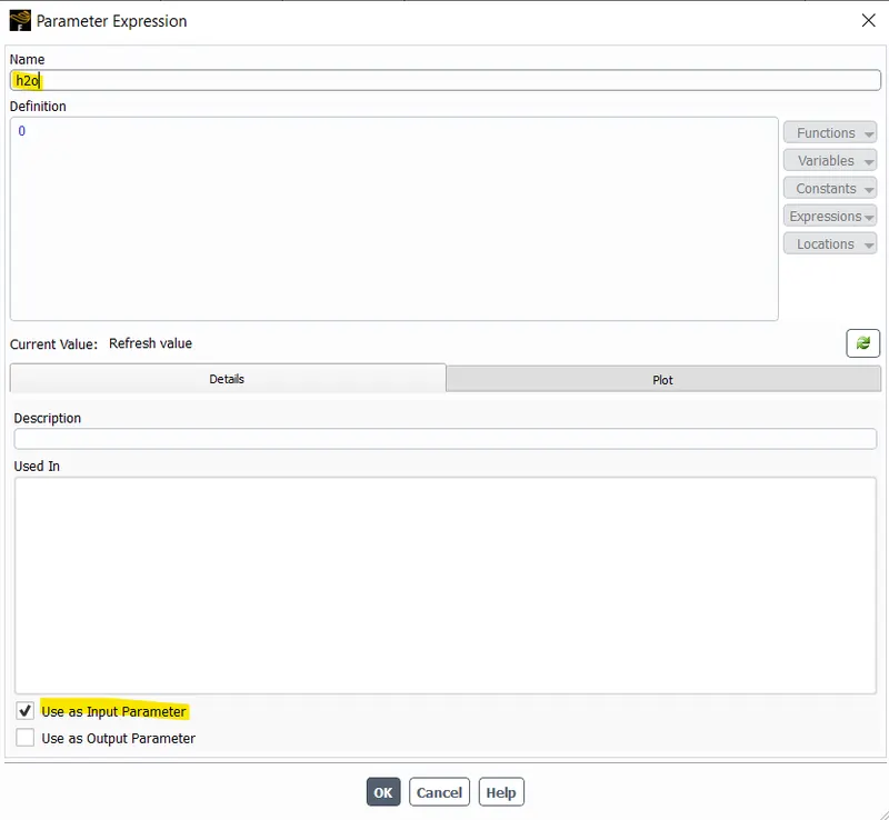
For part 2, The CH4 and H2O are made as the Input parameters.

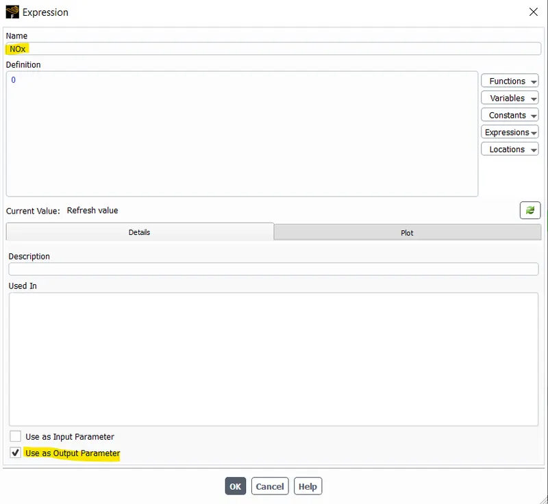
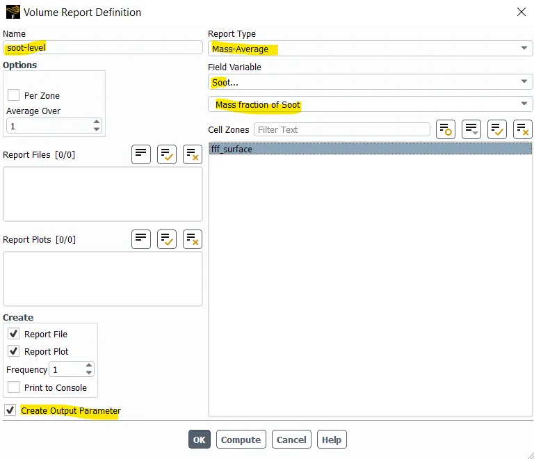
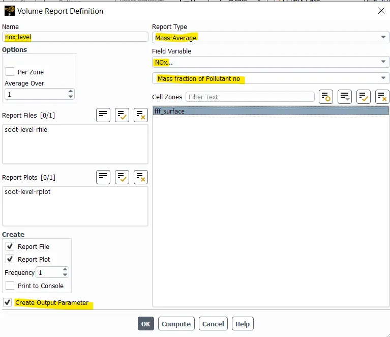
For part 2, the NOx and Soot level is given as the output parameters.

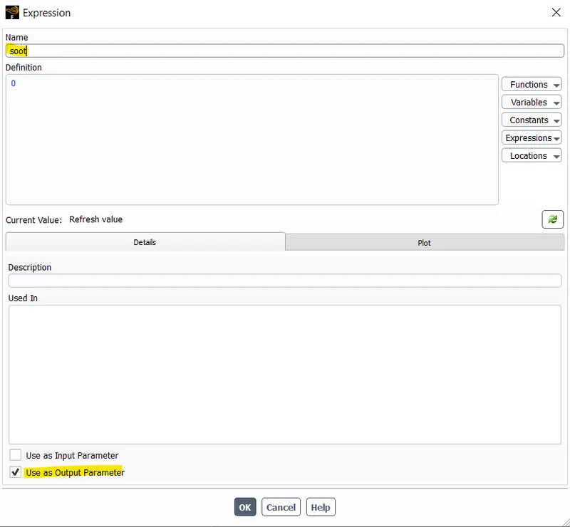
3.4: Boundary condition setup

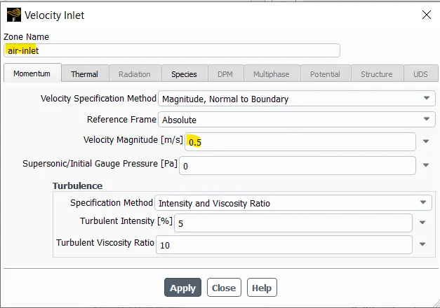
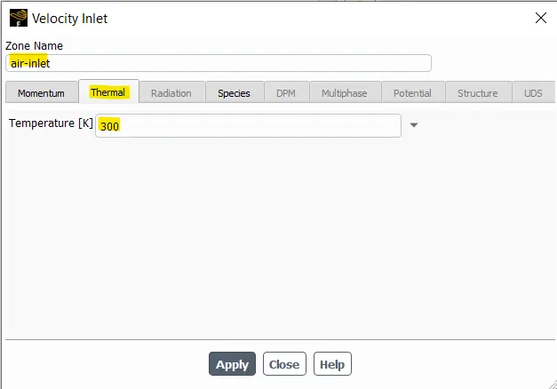
The inlet boundary conditions for air-inlet is set with 0.5m/s velocity, 300K temperature and the O2 mass fraction is set as 0.23 for all the cases.

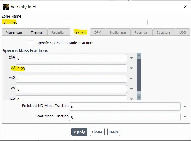
The inlet boundary condition for the fuel inlet is set with 80m/s velocity, 300K temperature and CH4 and H2O mass fractions.

For part 1 pure fuel, mass fraction of CH4 is given as 1.

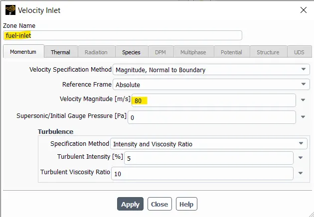
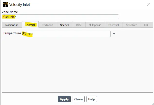
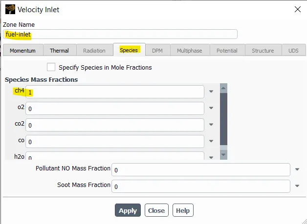
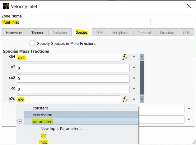
For part 2 fuel with inclusions, CH4 and H2O are given as the input parameters for which the value ranges between 0.95 - 0.7 and 0.05 - 0.3 respectively.

3.5: Report and definitions setup

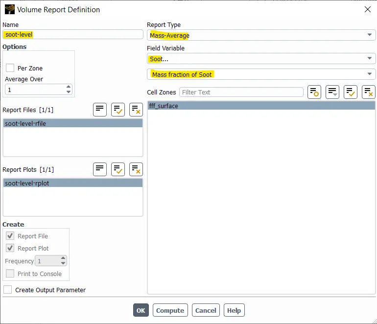
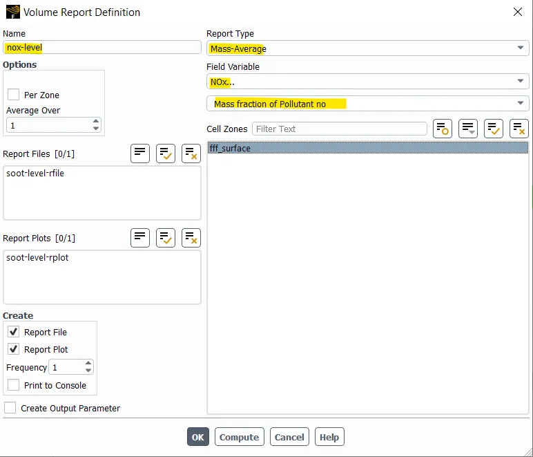
For part 1, NOx level and Soot level are given is definitions in the volume with a mass average report type.

For part 2, NOx level and Soot level are given in definitions in the volume with a mass average report and is made as the output parameters.

3.6: Residuals and initialization

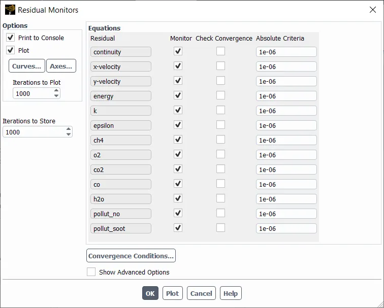
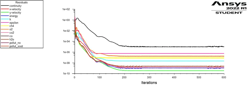
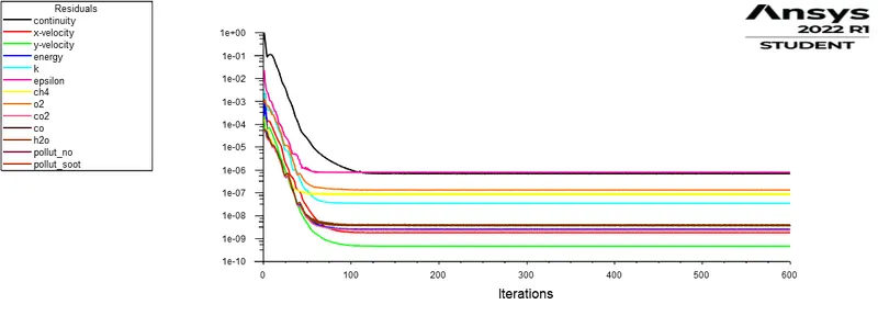
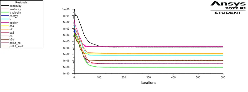
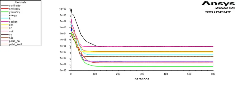
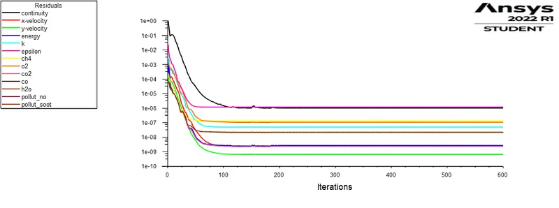
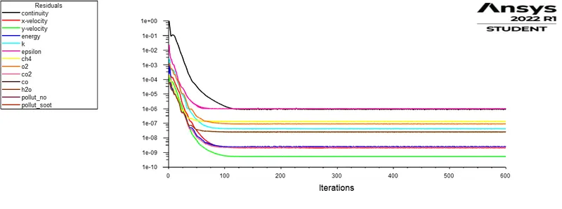
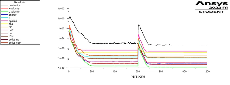
Finally, the residuals are checked, the convergence criteria is checked, hybrid initialization is done, and the solution is run for 600 iterations.

Step 4: Parameter assigning and post processing

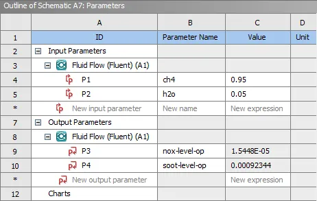
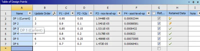
The CH4 and H2O percentage is assigned as the input parameter and Nox pollutant level and soot formation level is assigned as the output parameters for part 2 of the simulation. 6 design points with CH4 levels ranging from 0.95 to 0.7 and H2O levels ranging from 0.05 to 0.3 is created.

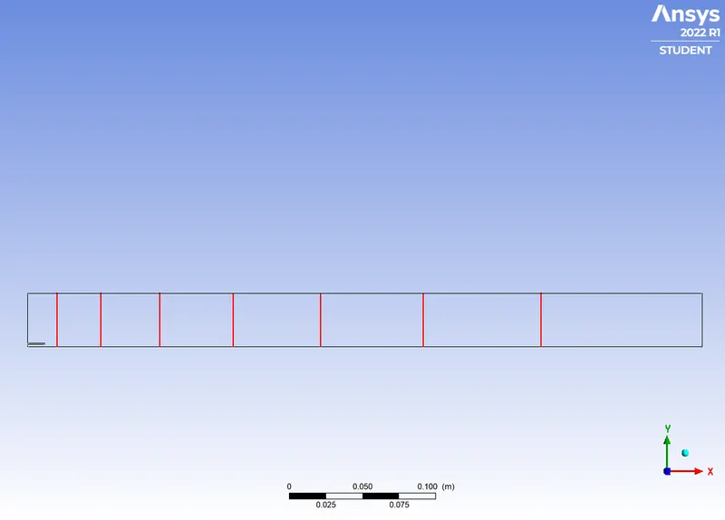
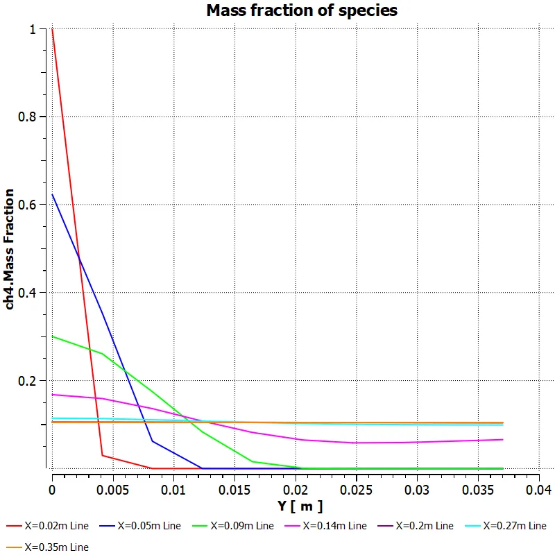
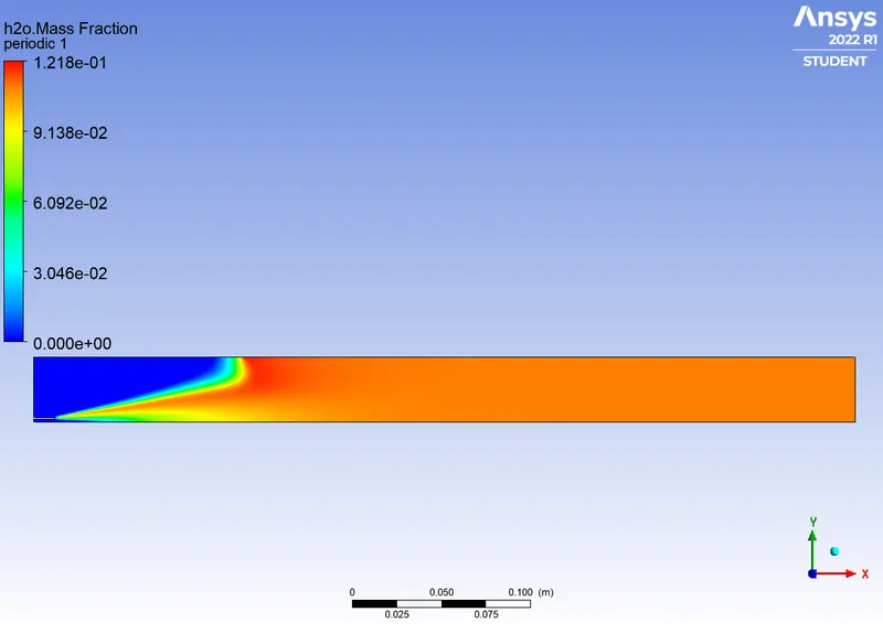
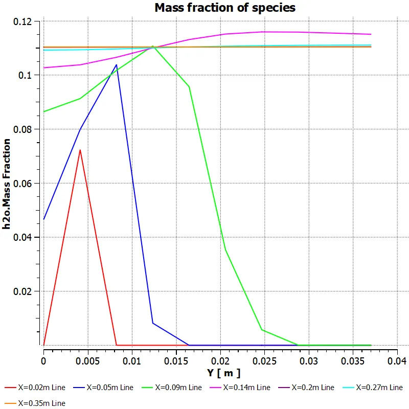
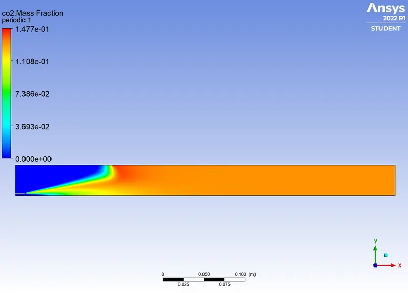
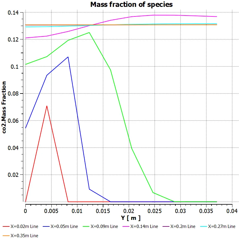
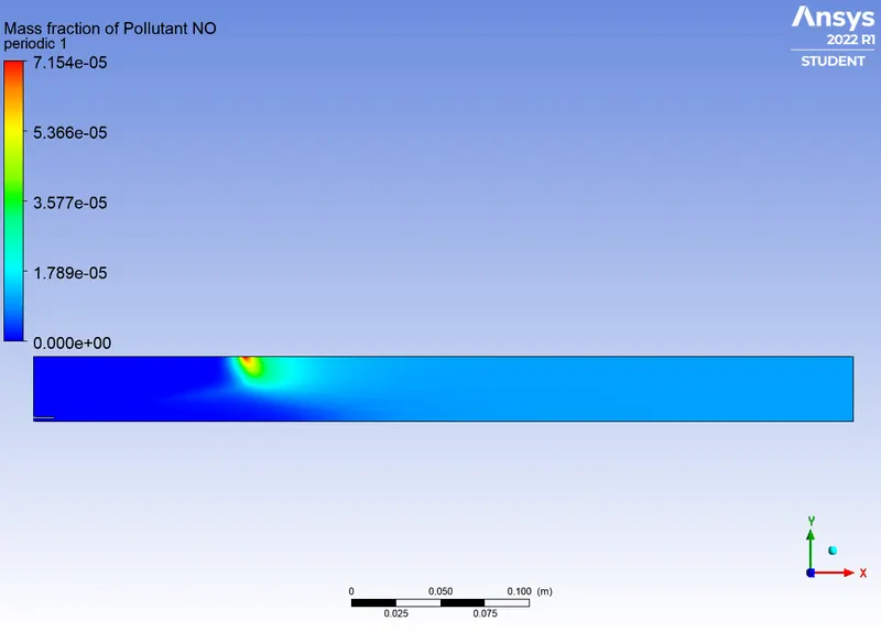
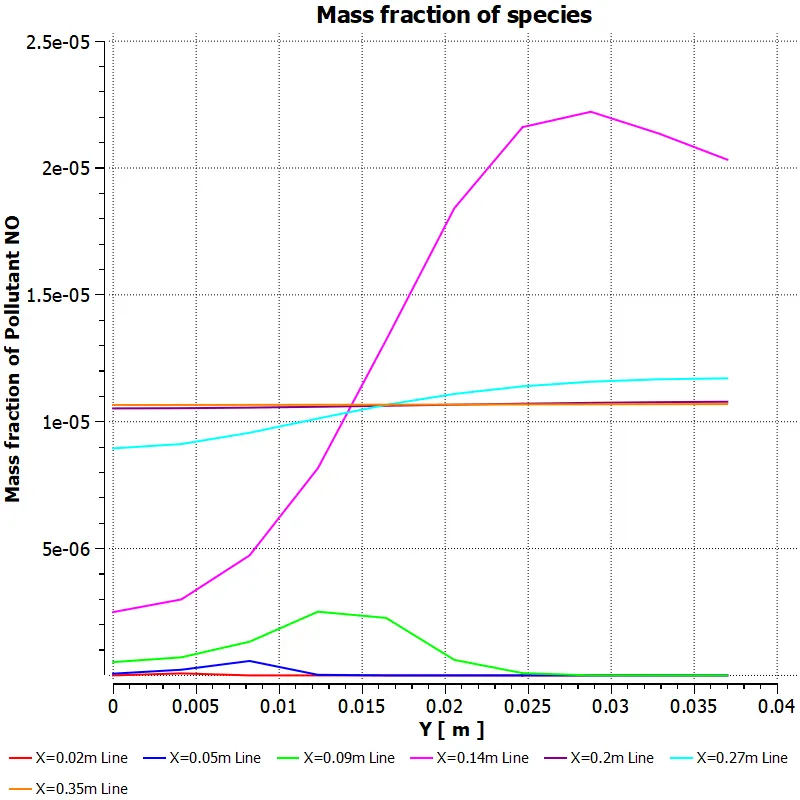
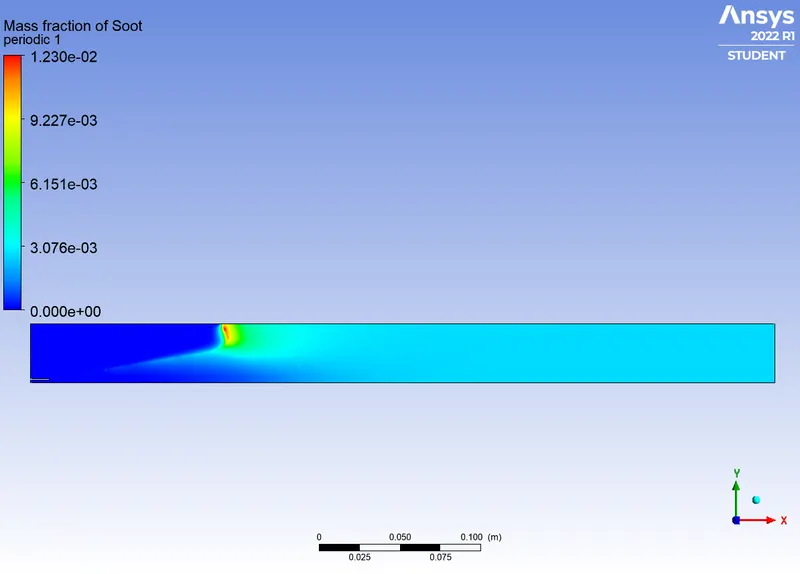
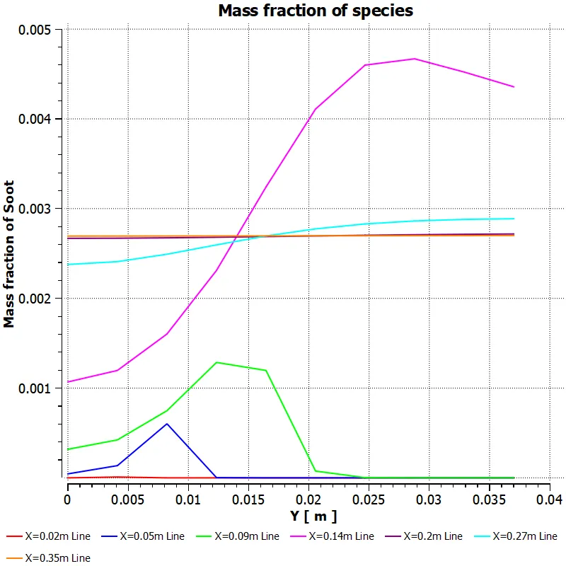
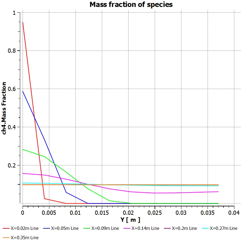
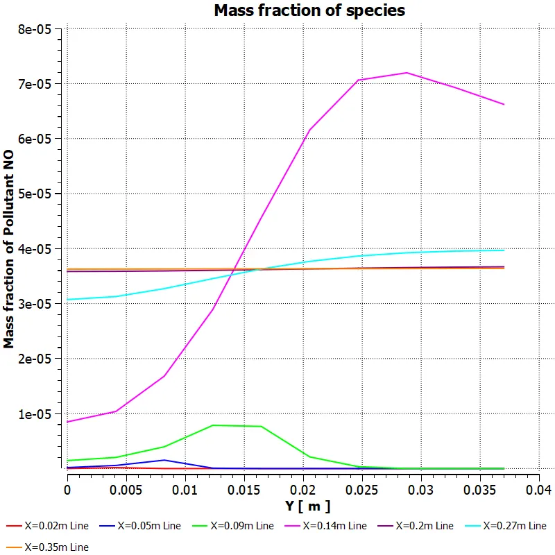
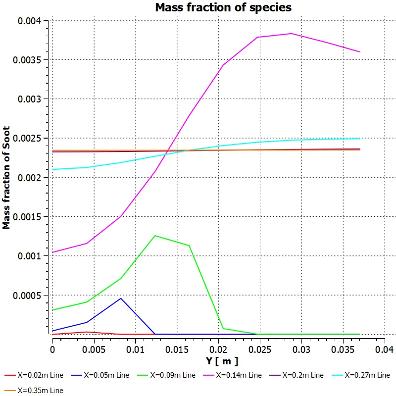
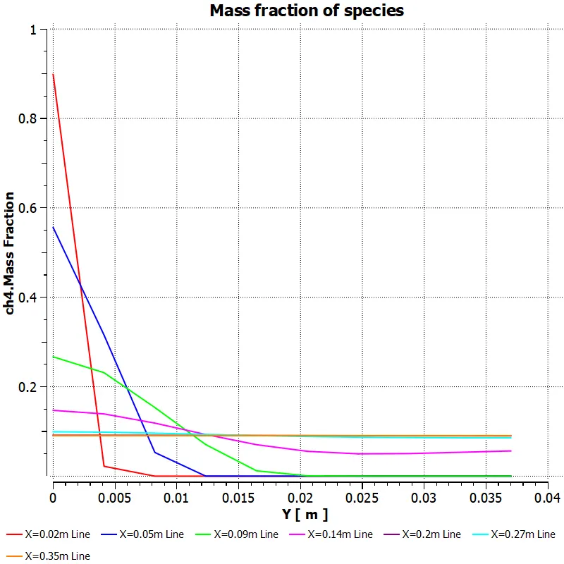
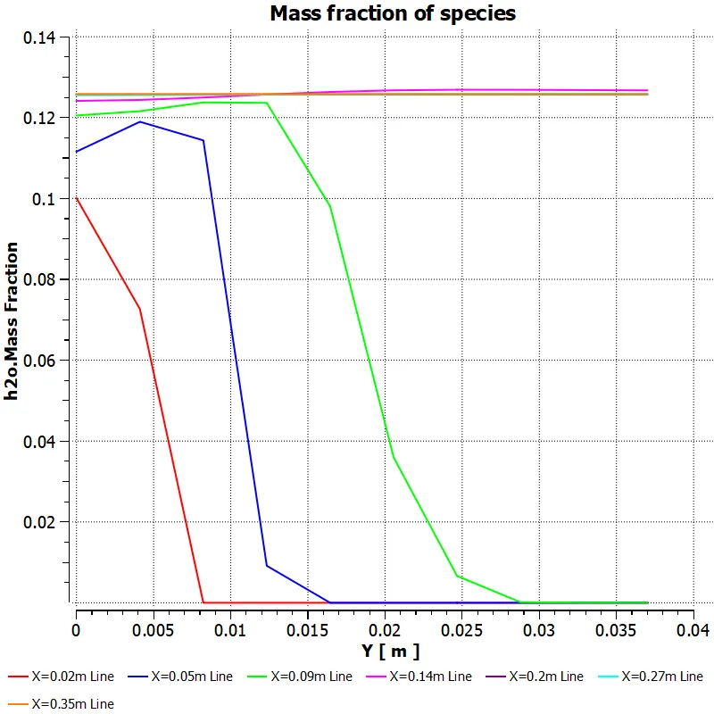
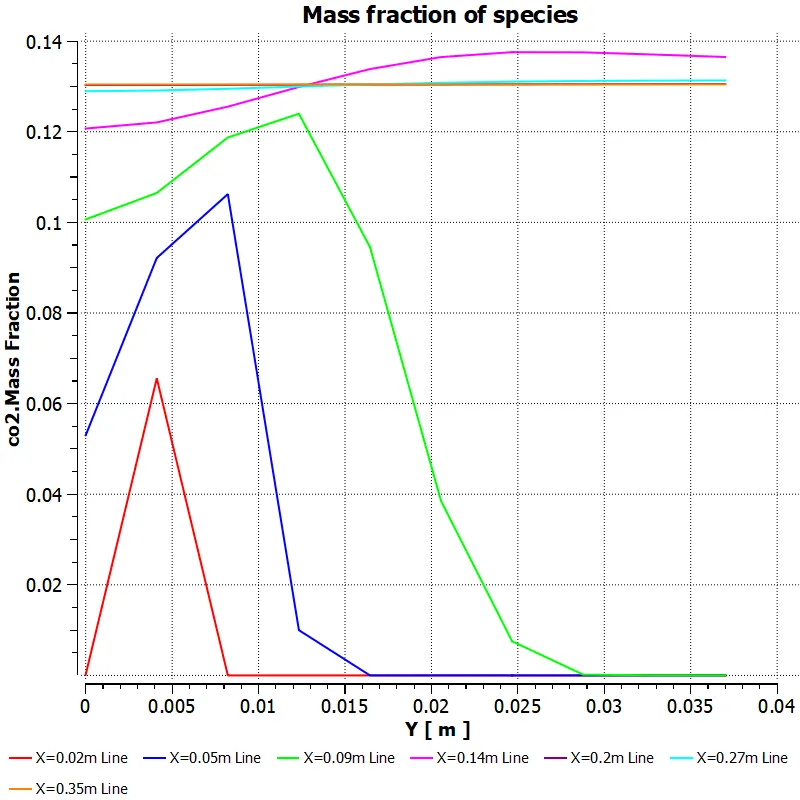
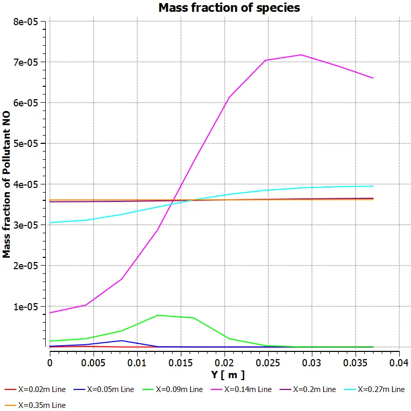
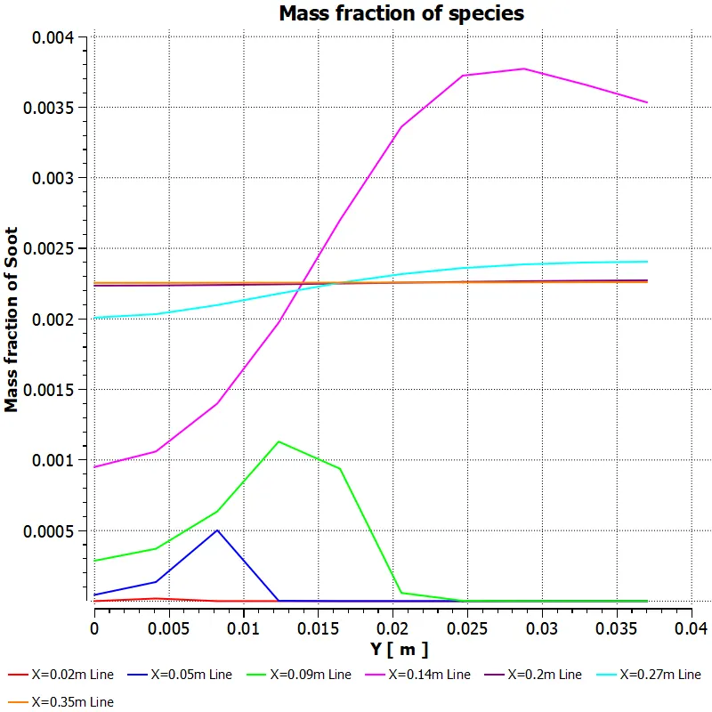
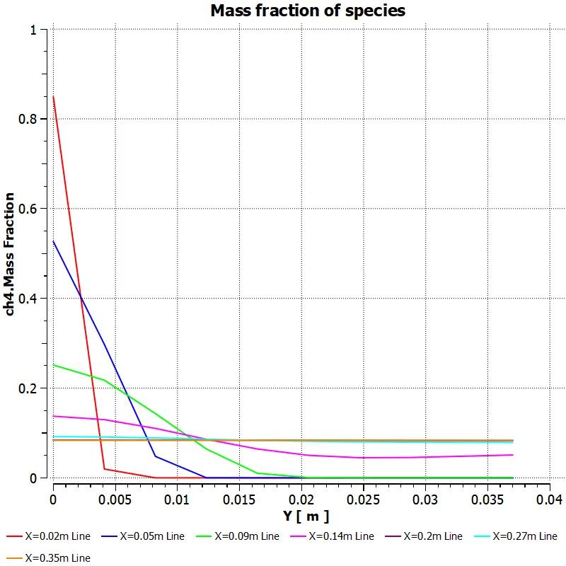
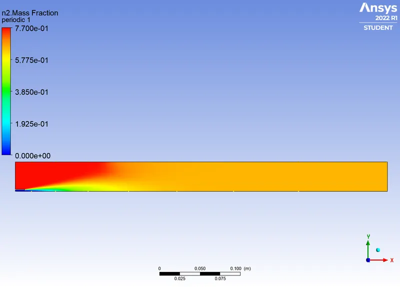
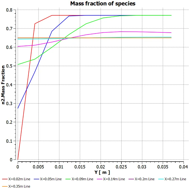
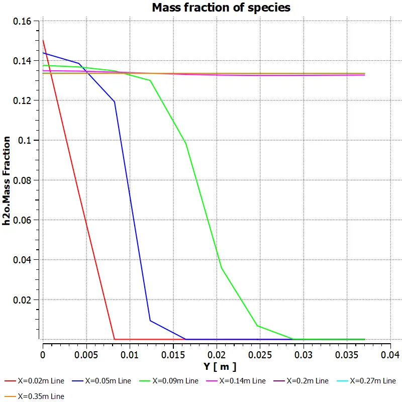
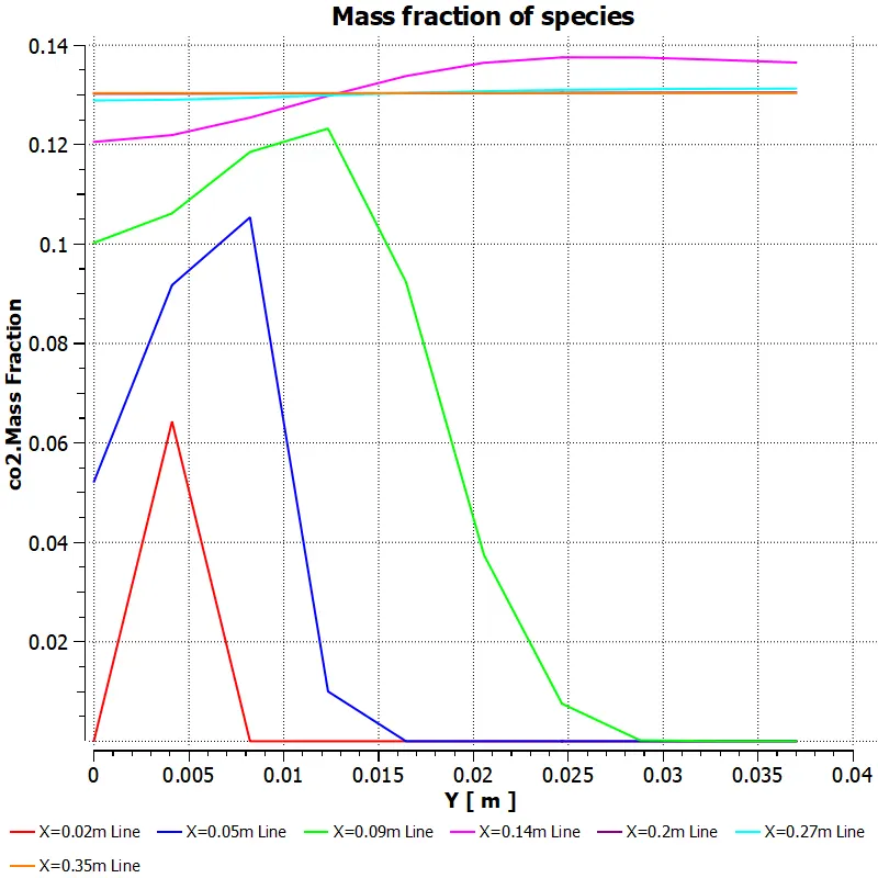
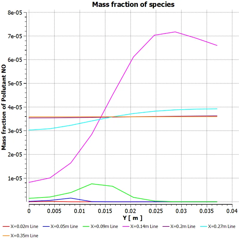
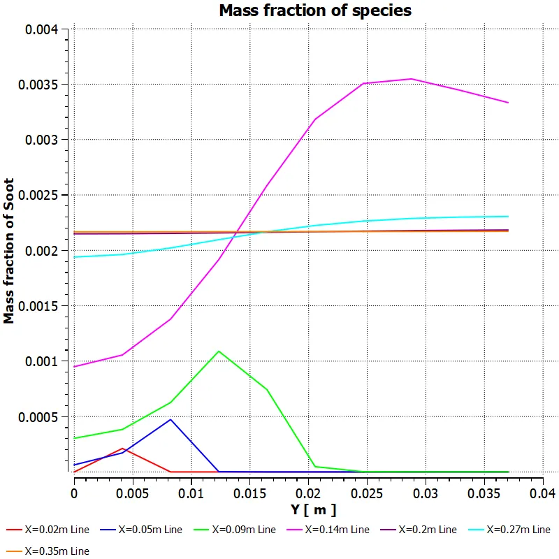
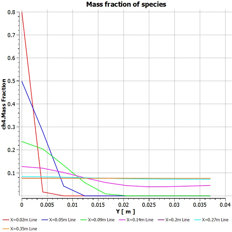
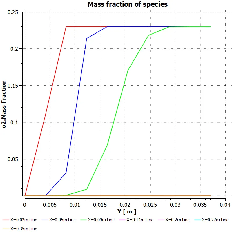
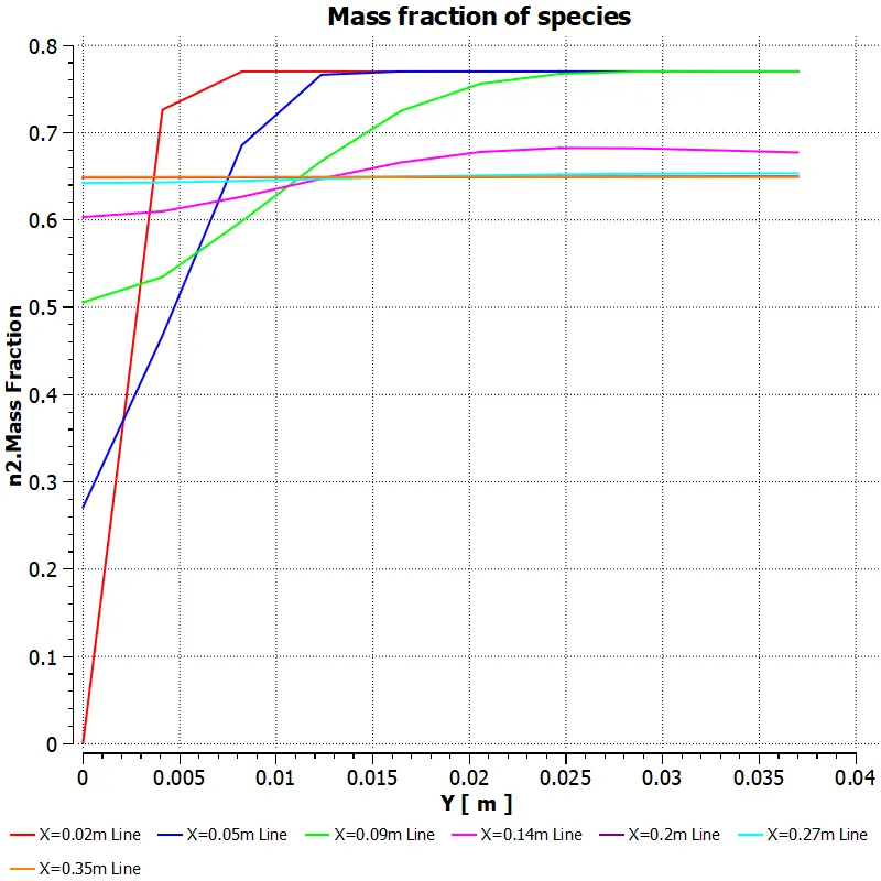
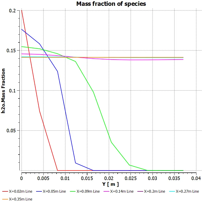
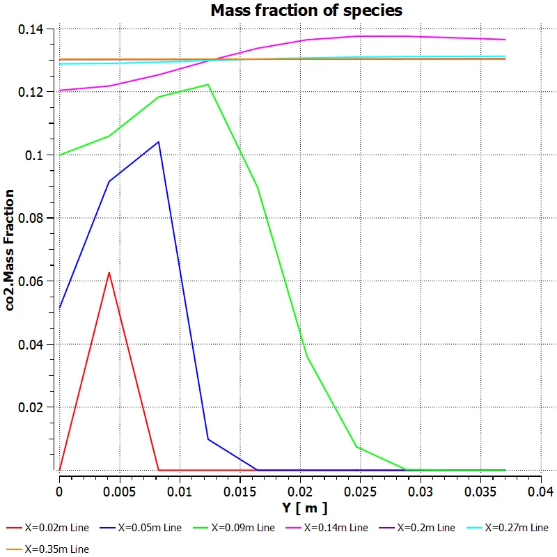
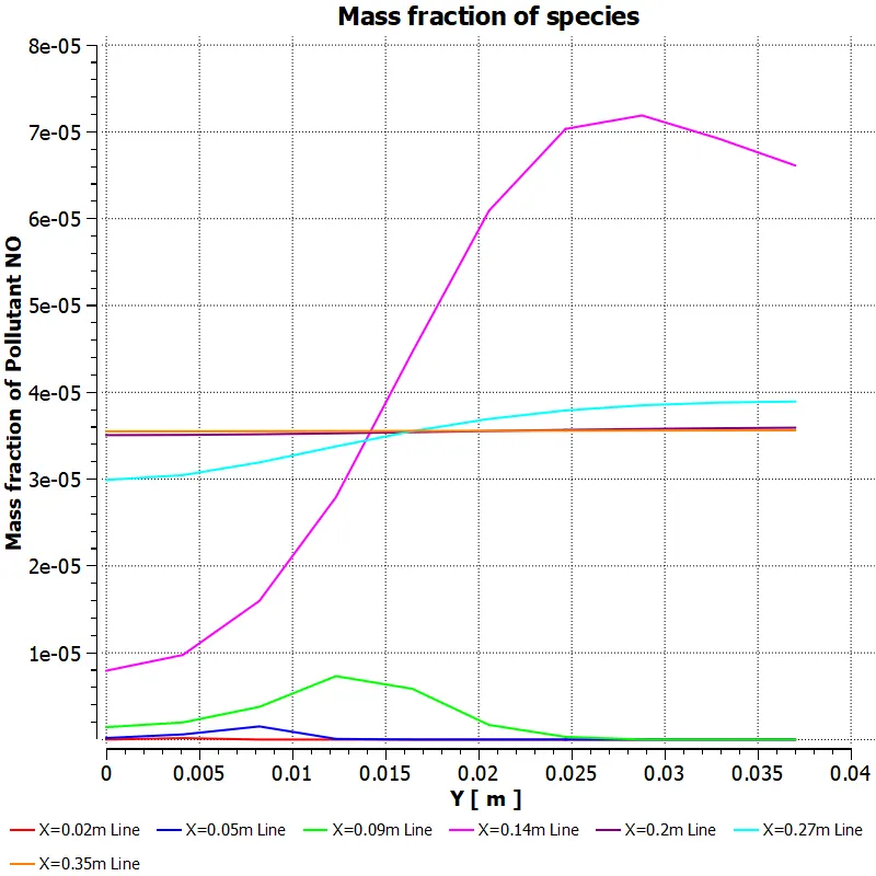
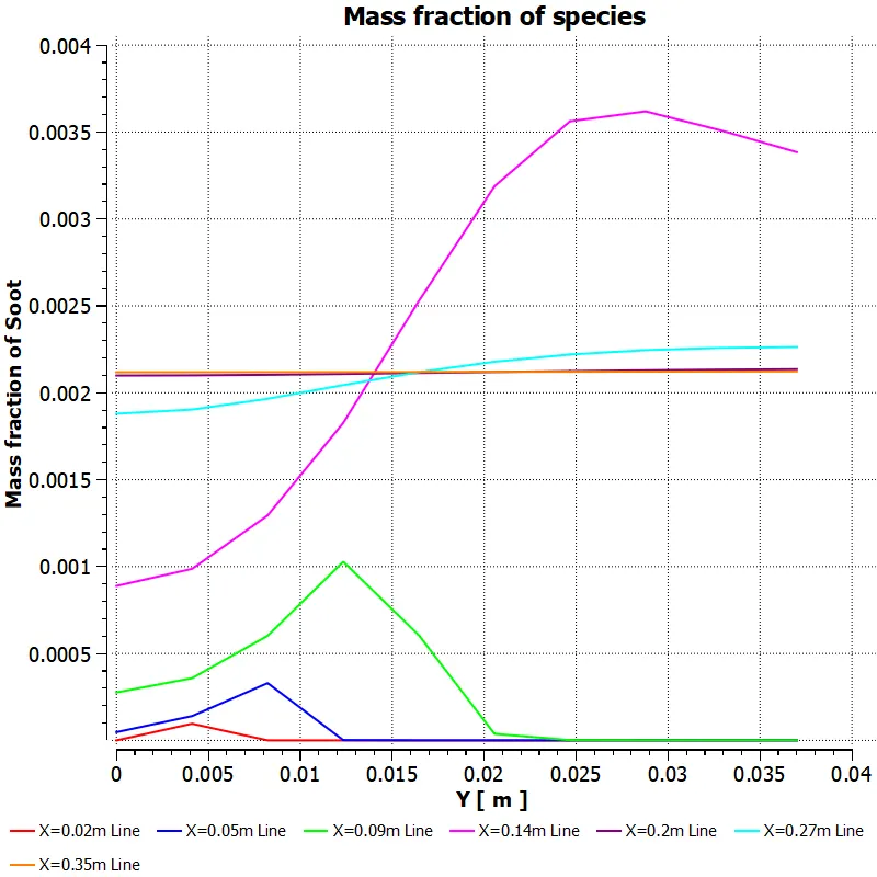
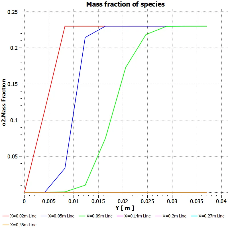
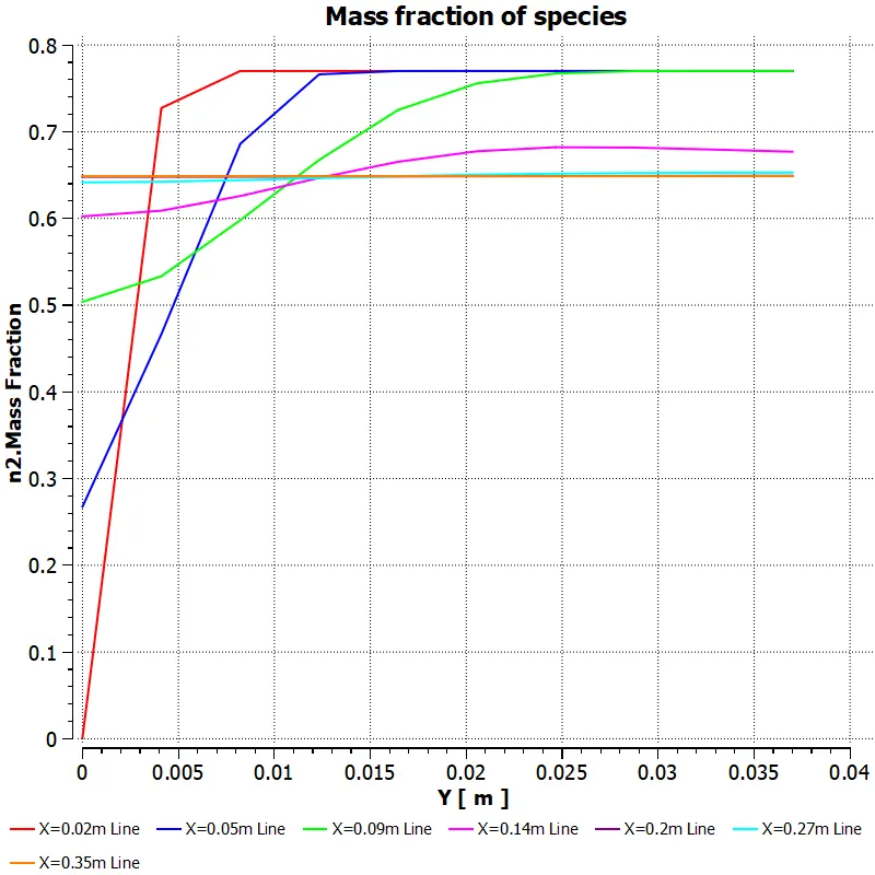
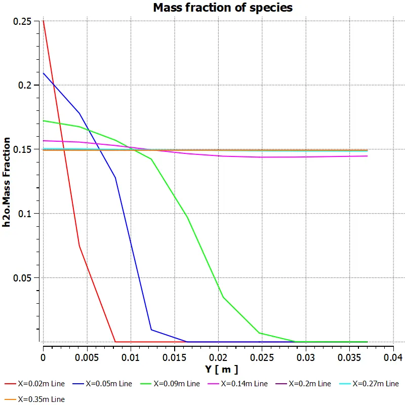
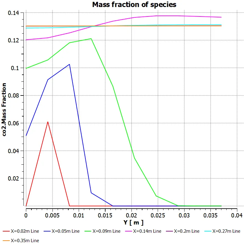
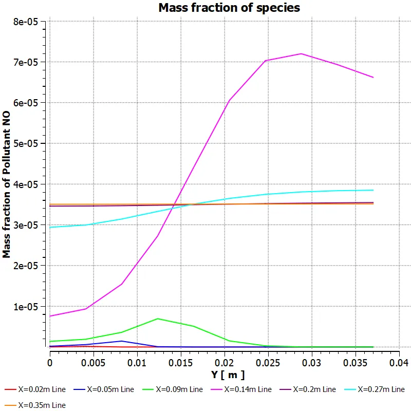
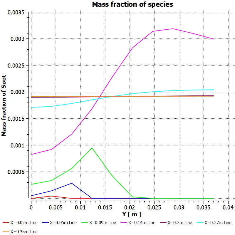
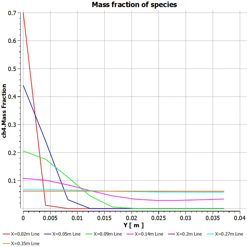
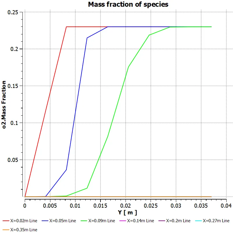
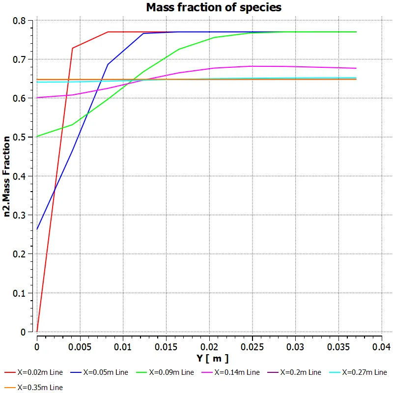
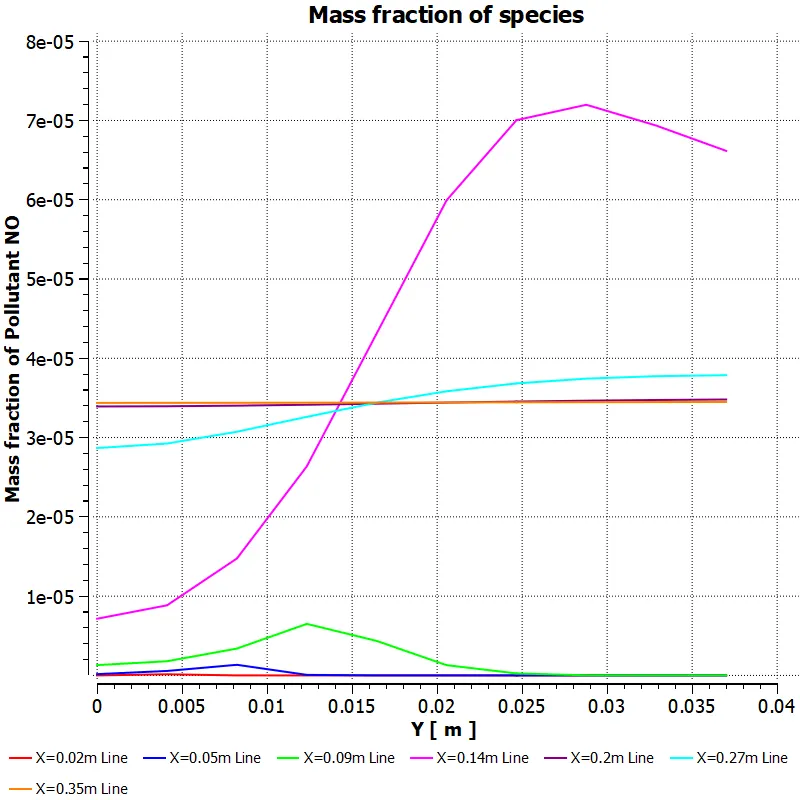
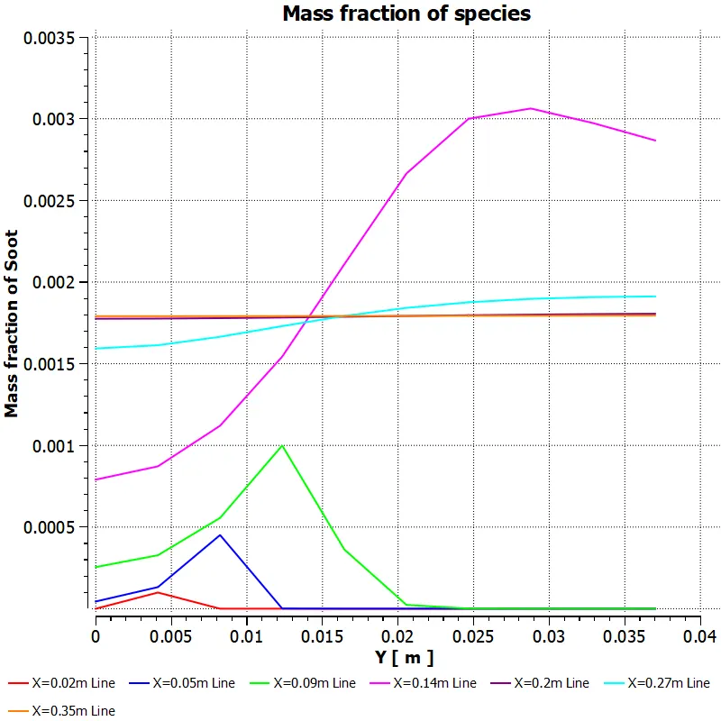
The line probes at various points at X= 0.02m, X=0.05m, X=0.09m, X=0.14m. X= 0.2m, X=0.27m, and X=0.35m are plotted and the charts are generated for various species in CFD Post. These lines are vertical X-lines used to study the variation of a particular property along the Y-axis. The charts are plotted with Y length units in the X-axis and the property in the Y-axis and the point locations are denoted by these lines.

Results:

Part 1: Pure CH4 fuel

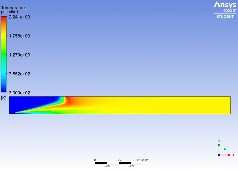
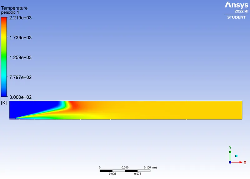
Residuals:	Temperature plot:
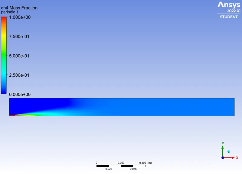
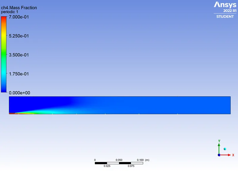
CH4 mass fraction plot:	CH4 mass fraction chart:
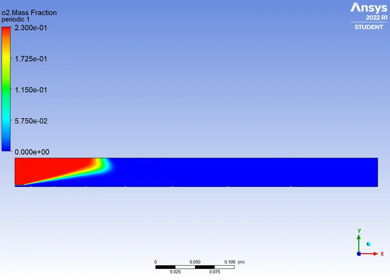
O2 mass fraction plot:	O2 mass fraction chart:
N2 mass fraction plot:	N2 mass fraction chart:
H2O mass fraction plot:	H2O mass fraction chart:
CO2 mass fraction plot:	CO2 mass fraction chart:
NOx pollutant mass fraction plot:	NOx pollutant mass fraction chart:
Soot mass fraction plot:	Soot mass fraction chart:

Part 2: CH4 fuel with H2O inclusions

Case 2.1: Fuel with 95% CH4 and 5% H2O

Residuals:	Temperature plot:
CH4 mass fraction plot:	CH4 mass fraction chart:
O2 mass fraction plot:	O2 mass fraction chart:
N2 mass fraction plot:	N2 mass fraction chart:
H2O mass fraction plot:	H2O mass fraction chart:
CO2 mass fraction plot:	CO2 mass fraction chart:
NOx pollutant mass fraction plot:	NOx pollutant mass fraction chart:
Soot mass fraction plot:	Soot mass fraction chart:

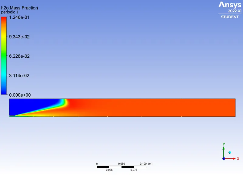
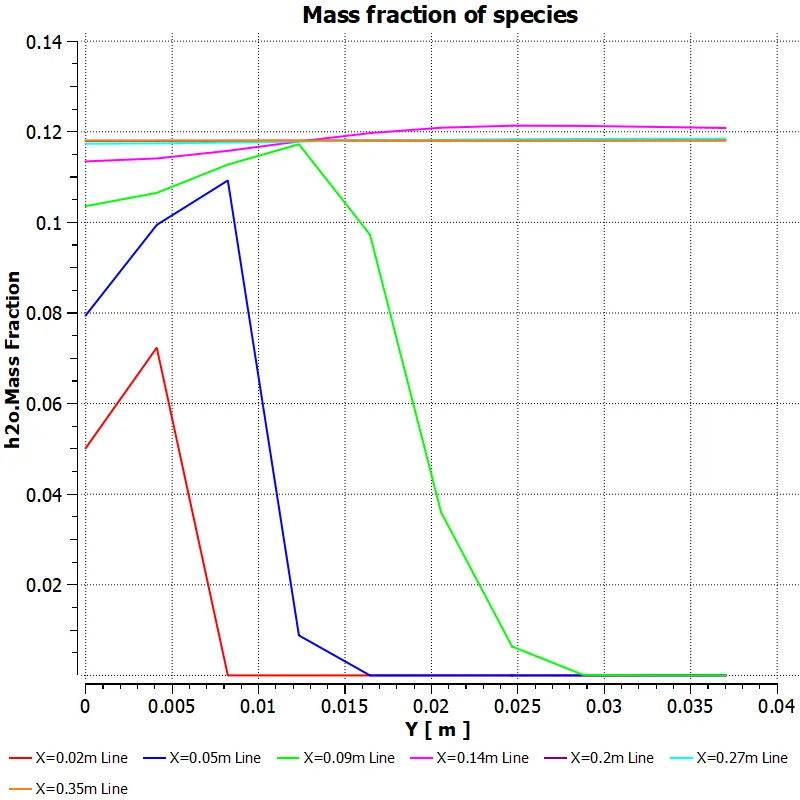
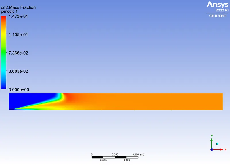
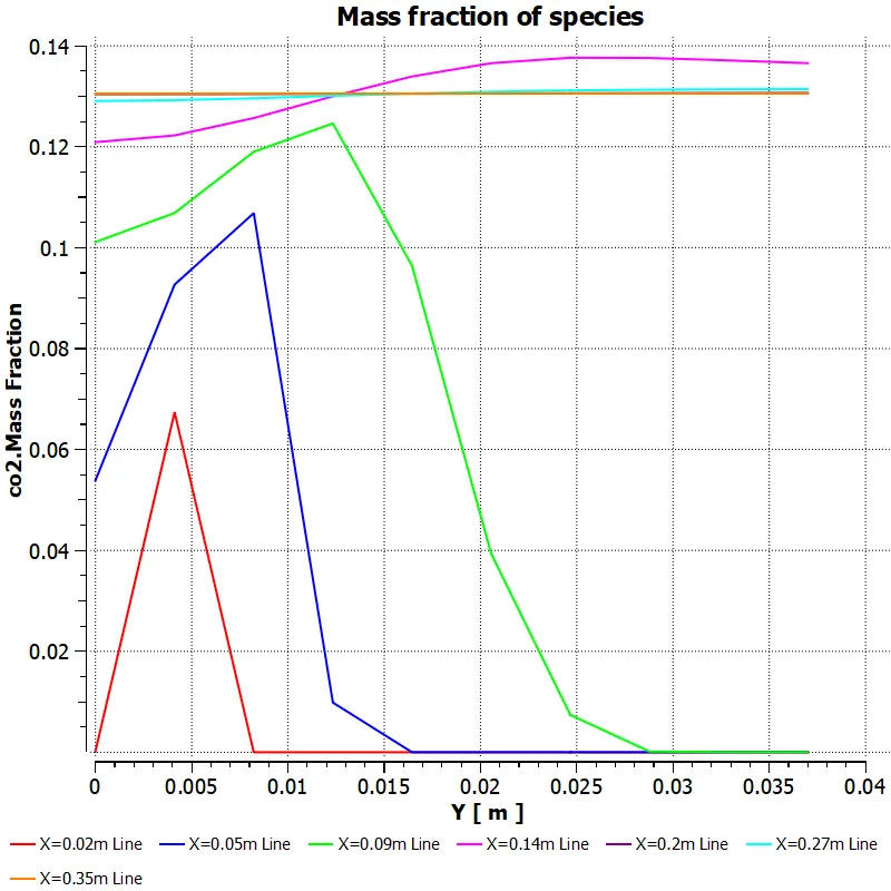
Case 2.2: Fuel with 90% CH4 and 10% H2O

Residuals:	Temperature plot:
CH4 mass fraction plot:	CH4 mass fraction chart:
O2 mass fraction plot:	O2 mass fraction chart:
N2 mass fraction plot:	N2 mass fraction chart:
H2O mass fraction plot:	H2O mass fraction chart:
CO2 mass fraction plot:	CO2 mass fraction chart:
NOx pollutant mass fraction plot:	NOx pollutant mass fraction chart:
Soot mass fraction plot:	Soot mass fraction chart:

Case 2.3: Fuel with 85% CH4 and 15% H2O

Residuals:	Temperature plot:
CH4 mass fraction plot:	CH4 mass fraction chart:
O2 mass fraction plot:	O2 mass fraction chart:
N2 mass fraction plot:	N2 mass fraction chart:
H2O mass fraction plot:	H2O mass fraction chart:
CO2 mass fraction plot:	CO2 mass fraction chart:
NOx pollutant mass fraction plot:	NOx pollutant mass fraction chart:
Soot mass fraction plot:	Soot mass fraction chart:

Case 2.4: Fuel with 80% CH4 and 20% H2O

Residuals:	Temperature plot:
CH4 mass fraction plot:	CH4 mass fraction chart:
O2 mass fraction plot:	O2 mass fraction chart:
N2 mass fraction plot:	N2 mass fraction chart:
H2O mass fraction plot:	H2O mass fraction chart:
CO2 mass fraction plot:	CO2 mass fraction chart:
NOx pollutant mass fraction plot:	NOx pollutant mass fraction chart:
Soot mass fraction plot:	Soot mass fraction chart:

Case 2.5: Fuel with 75% CH4 and 25% H2O

Residuals:	Temperature plot:
CH4 mass fraction plot:	CH4 mass fraction chart:
O2 mass fraction plot:	O2 mass fraction chart:
N2 mass fraction plot:	N2 mass fraction chart:
H2O mass fraction plot:	H2O mass fraction chart:
CO2 mass fraction plot:	CO2 mass fraction chart:
NOx pollutant mass fraction plot:	NOx pollutant mass fraction chart:
Soot mass fraction plot:	Soot mass fraction chart:

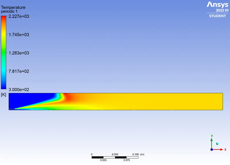
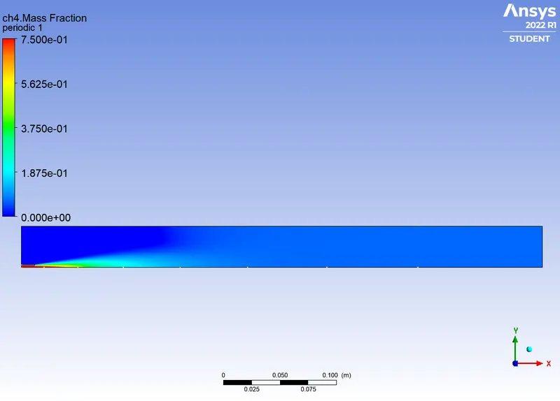
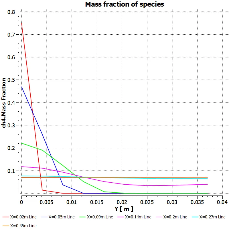
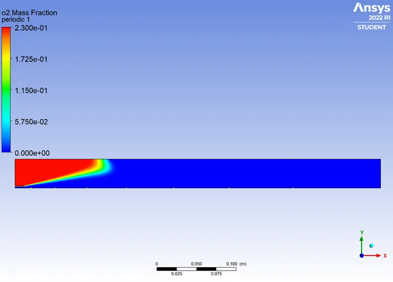
Case 2.6: Fuel with 70% CH4 and 30% H2O

Residuals:	Temperature plot:
CH4 mass fraction plot:	CH4 mass fraction chart:
O2 mass fraction plot:	O2 mass fraction chart:
N2 mass fraction plot:	N2 mass fraction chart:
H2O mass fraction plot:	H2O mass fraction chart:
CO2 mass fraction plot:	CO2 mass fraction chart:
NOx pollutant mass fraction plot:	NOx pollutant mass fraction chart:
Soot mass fraction plot:	Soot mass fraction chart:

Computed values:

Inference:

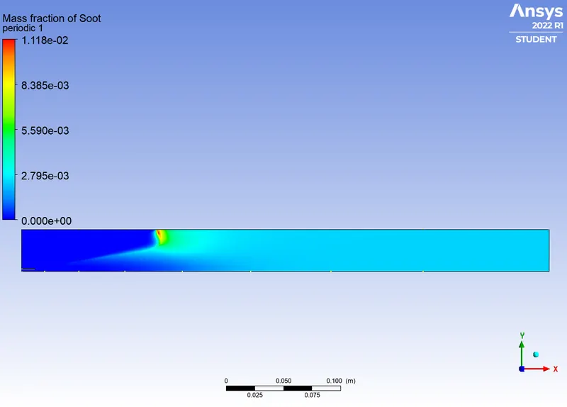
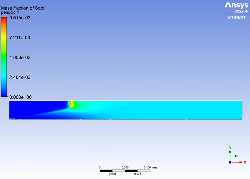
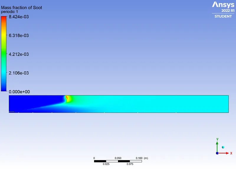
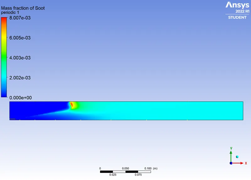
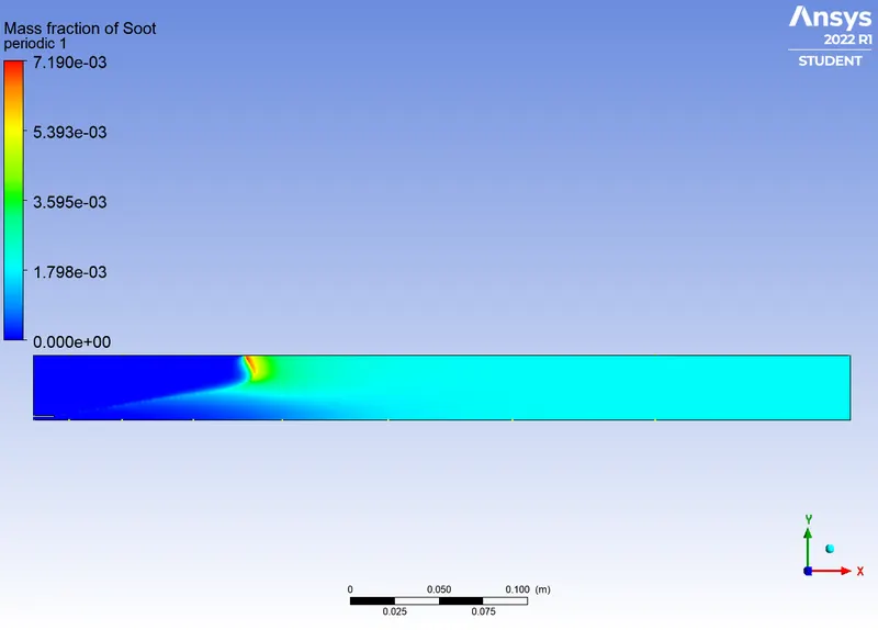
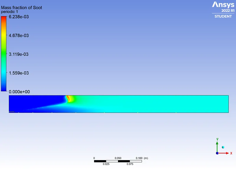
The combustion model simulated contains a mixture of N2, CO2, H2O NOx and soot concentration. The emission of particulate matter or soot can be considered as a side effect of high temperature and rich fuel mixture conditions. Radiative heat transfer and soot volume fraction are monitored to determine the effectiveness. Soot production in methane-air flames usually takes place from small species like acetylene that grow to form polyaromatic hydrocarbons and eventually soot. The soot containing particles ranging between 5 nm to 100 nm is considered to be in the Rayleigh regime. Categories of models include empirical, semi-empirical and detailed models neglecting particle growth and its oxidation rates.

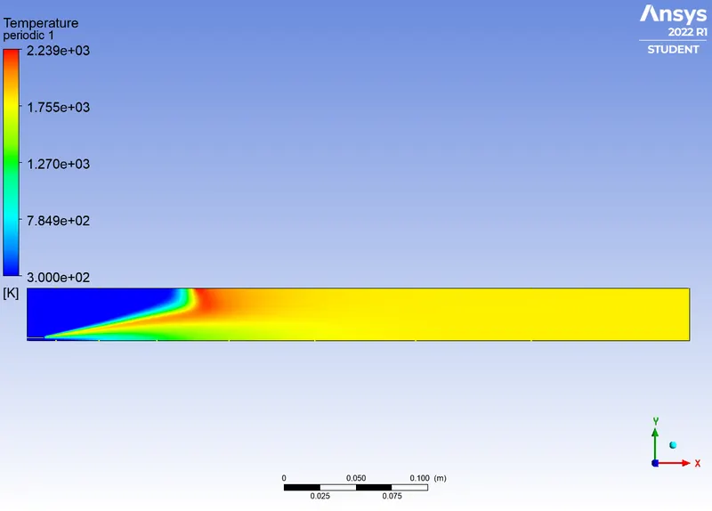
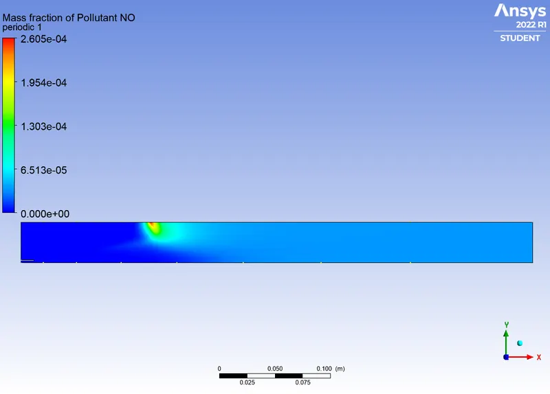
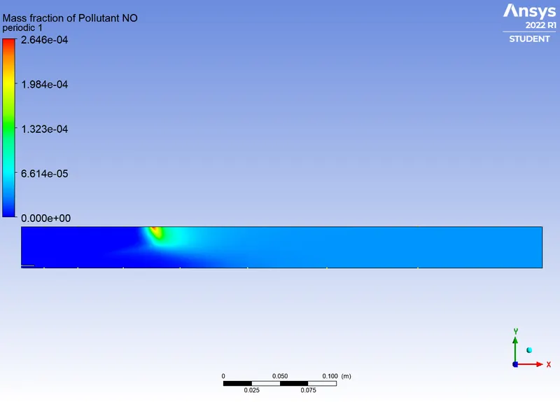
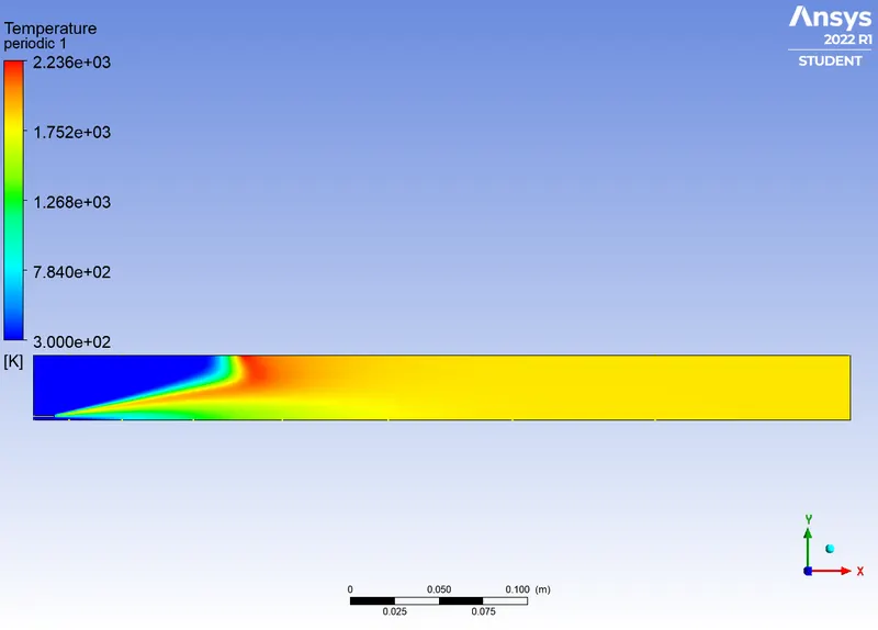
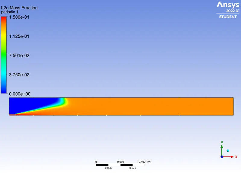
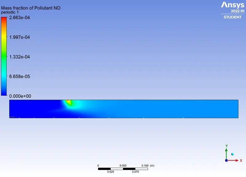
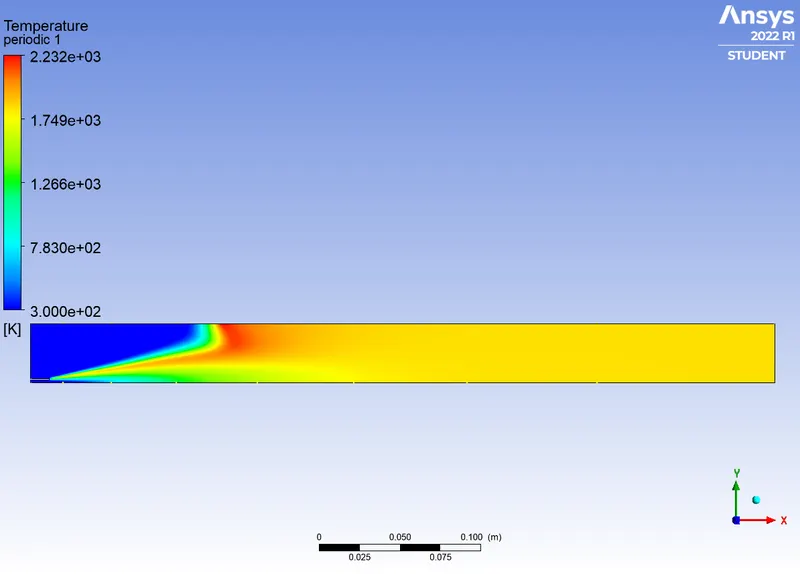
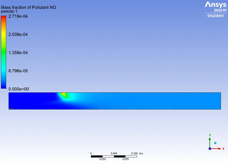
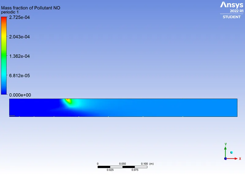
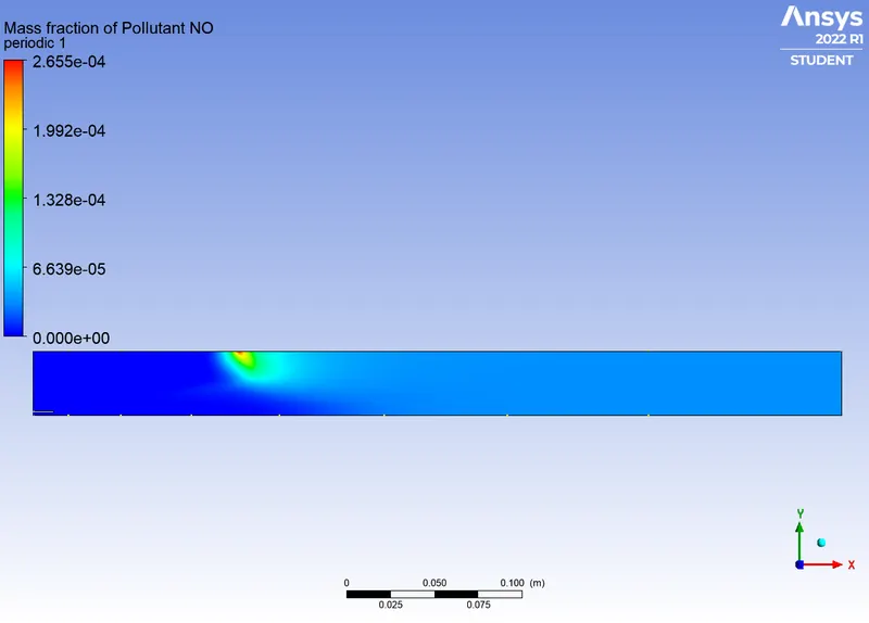
From the results, it is evident that the NOx level reduces when the composition of H2O in the fuel increases. A variety of methods have been employed to use water with the fuels inside the combustion chamber like continuous water injection and accumulated water cooled residual gas. Water should be demineralized to get rid of salts like sodium. Water supplied in the combustion chamber reduces the combustion temperature also. Using high pressure water injection, 25% of NOx content and 40% soot concentration is reduced in the emission gas. The NOx released is either due to oxidizing atmospheric nitrogen or oxidizing the nitrogen compounds present in the fuel. Due to the mixing of fuel and atmospheric air, the difference of velocity makes the NOx accumulate near the wall, where the two fluid streams combine the formation of eddies is seen.

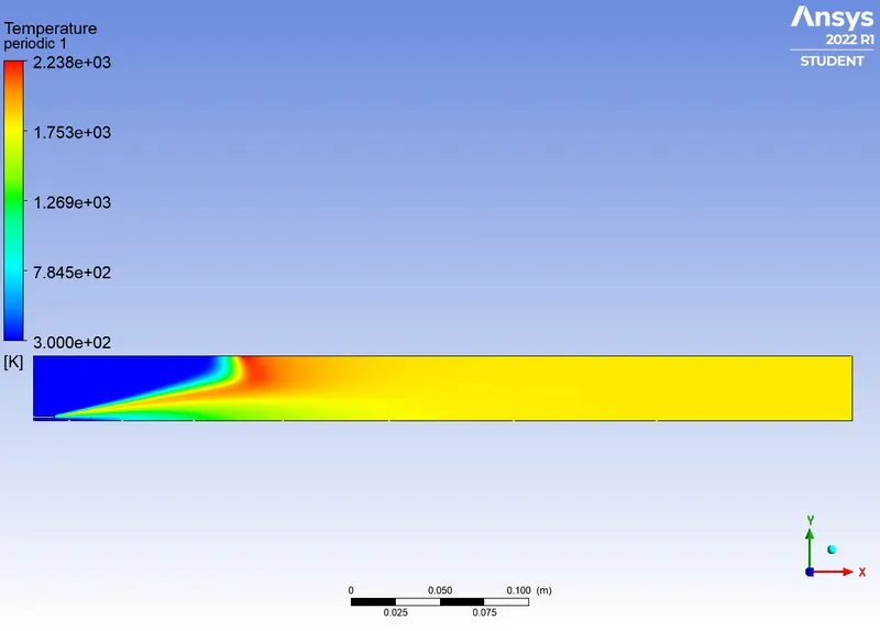
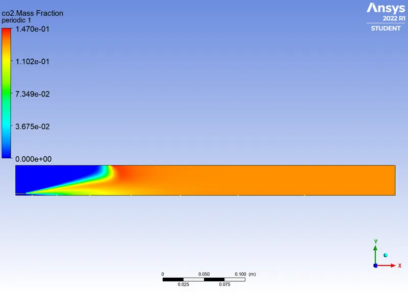
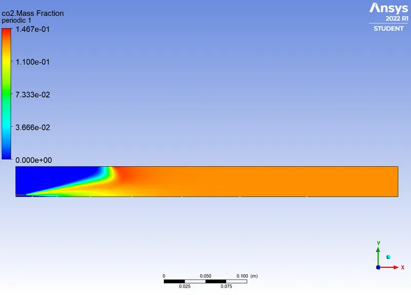
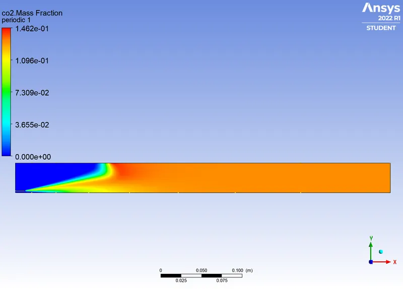
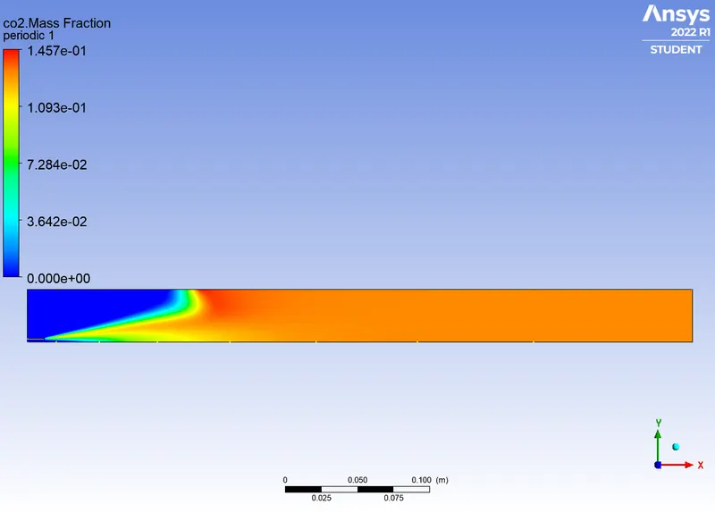
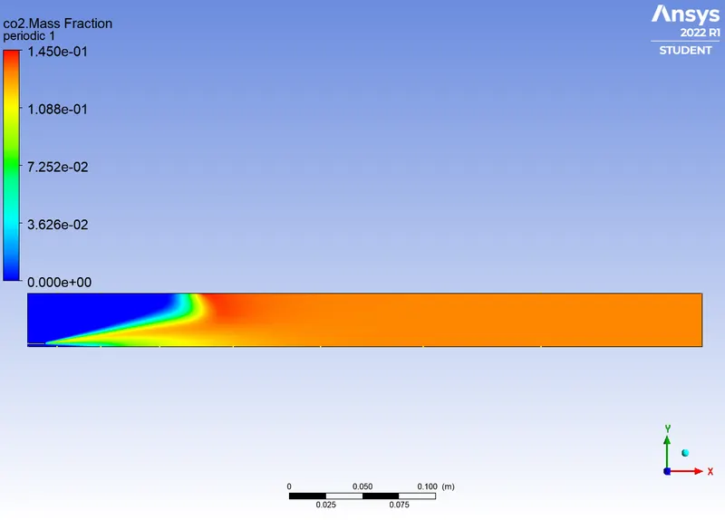
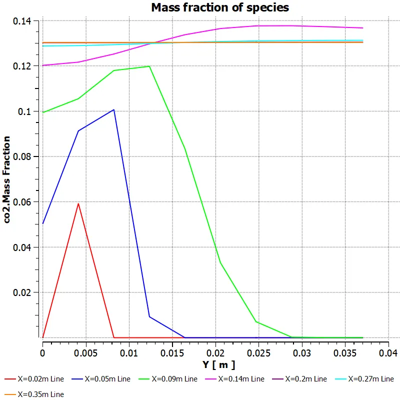
The appearance of CO2 is surely due to partially incomplete reaction, hence the stoichiometric mixture of reactants does not involve necessarily a complete reaction, an excess of air is always necessary to complete the combustion. CO2 is also considered as a polluting component. Once atmospheric air mixes with fuel there is temperature change and the composition of the CO2 increases at the interface and the balance fuel is thoroughly mixed, which can be observed at the outlet there is an uniform composition of the compounds.

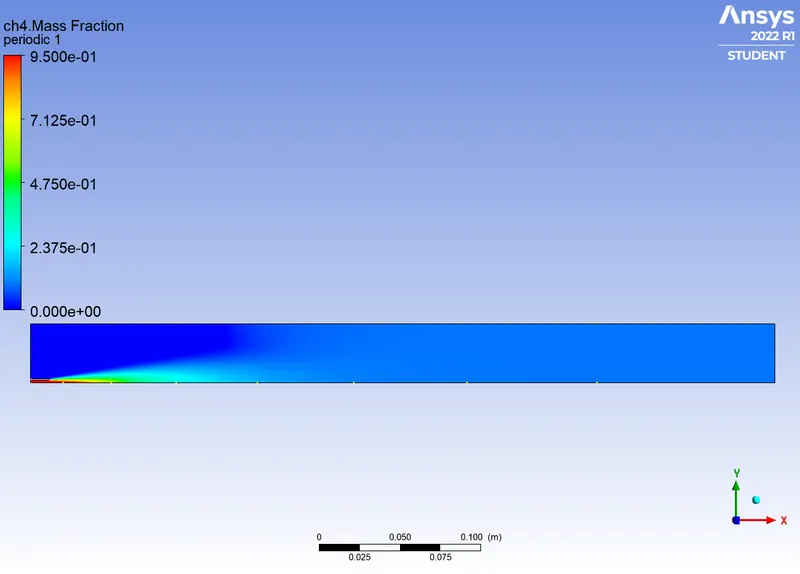
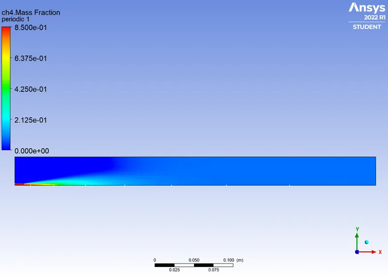
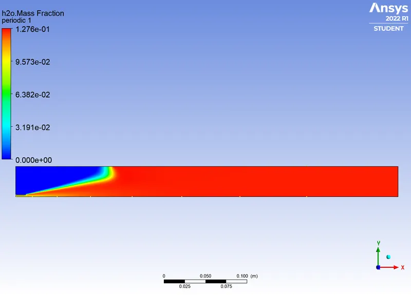
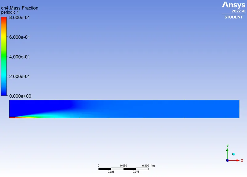
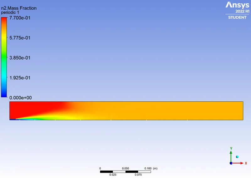
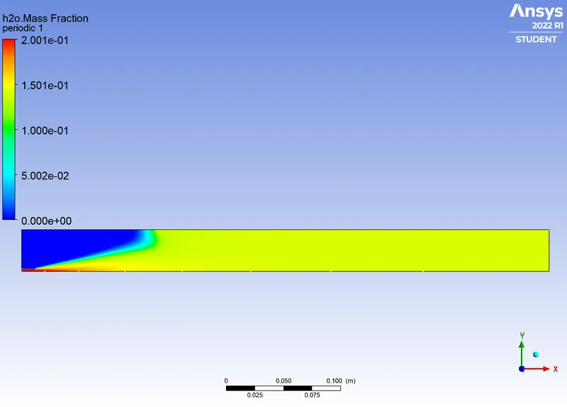
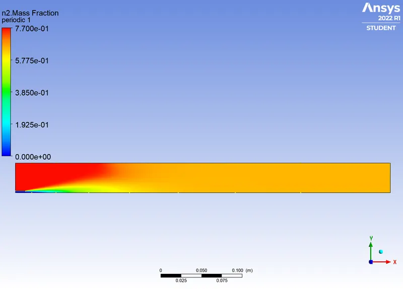
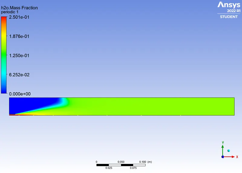
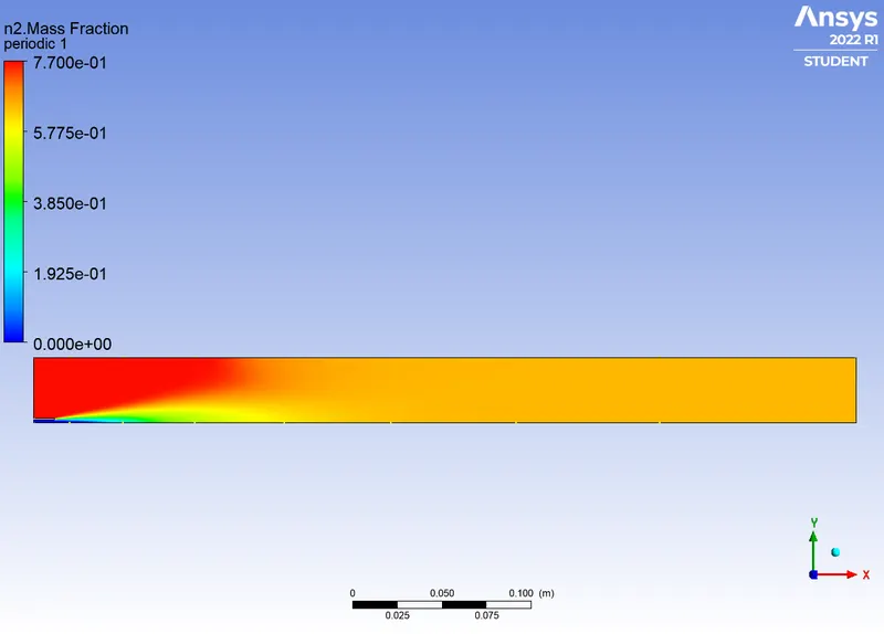
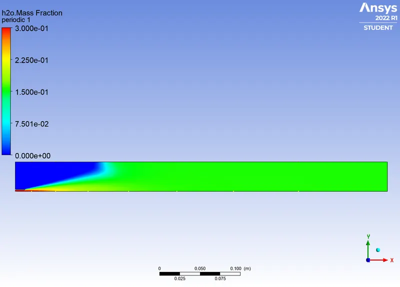
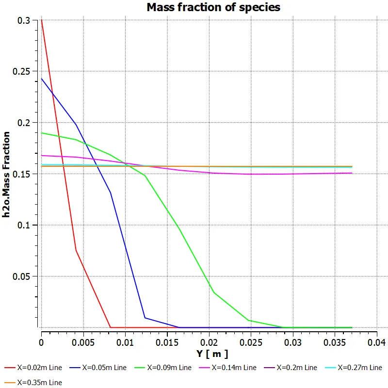
The H2O compounds is detected from the fuel inlet alone and hence undergoes a rapid mixing but is observed a uniform concentration at the outlet. The N2 compound in the oxidants is combusted from the inlet also, as the inlet air contains atmospheric nitrogen. This compound mixes with the fuel and hence mixes at the interface and oxidized uniformly in the outlet. The CH4 composition is completely due to the fuel and completely oxidized observed at the outlet.

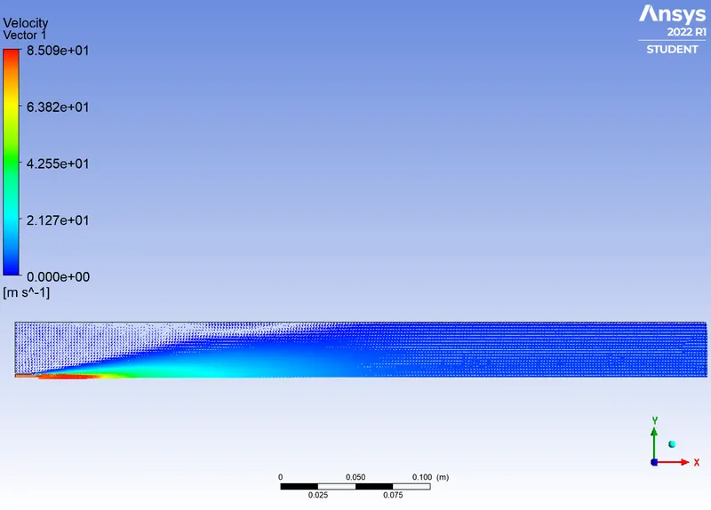
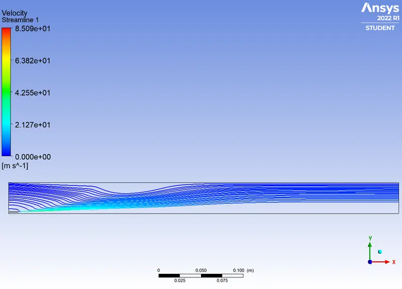
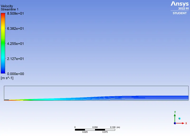
The velocity plots are also studied to analyse the mixing of fluid in relation to the geometry of the combustion chamber. Since there is a difference of velocity of the fluid streams, the mixing of fluid streams can be seen undergoing a laminar mixing, which then turns completely miscible in the outlet.

Conclusion:

The flow rate, temperature and mass fraction of individual species are used along with pressure outlet boundary condition. Since it is a combustion and eddy dissipation model, a false time stepping is followed to obtain a converged solution with a relaxation factor of 1e-6 with a mesh insensitive solution. The results are in accordance with the steady laminar flamelet model. The results are used to determine the effectiveness of pollution levels and combustion completeness.