Week 10 - Simulating Combustion of Natural Gas.

Aim:

Perform a combustion simulation on the combustor model using Methane gas.

objective:

Part I

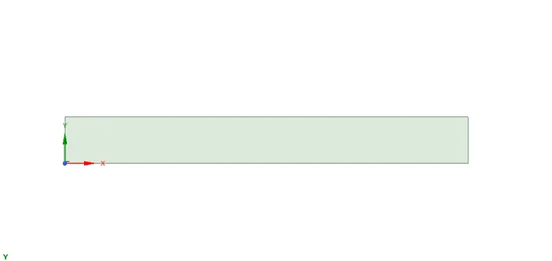
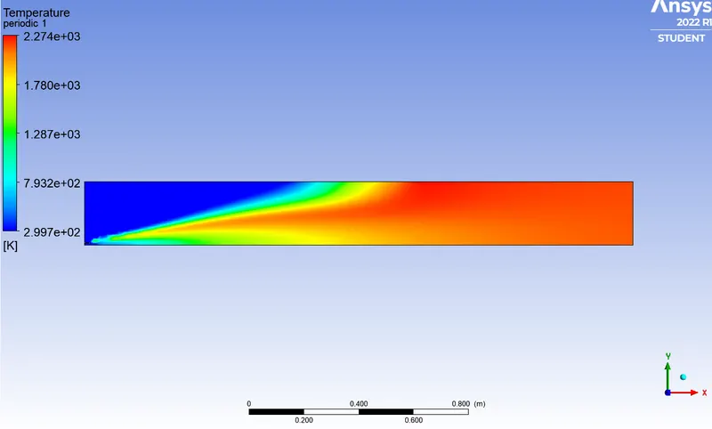
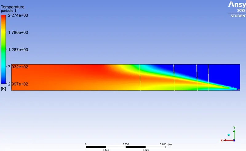
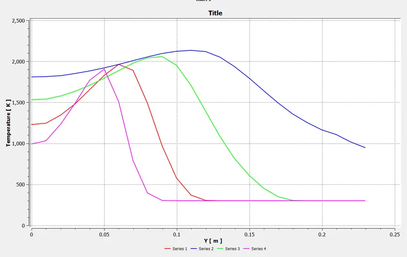
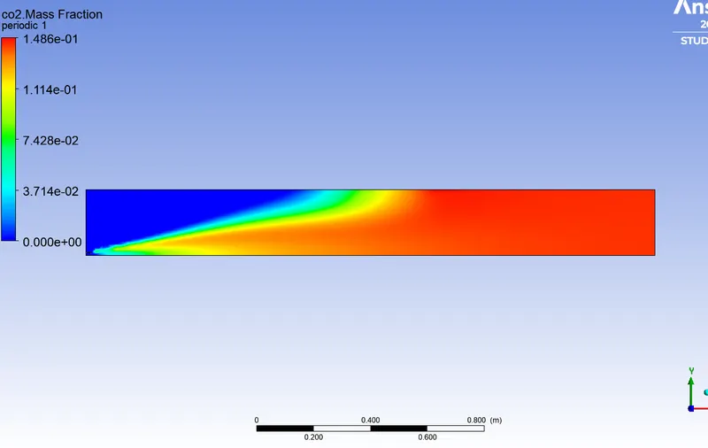
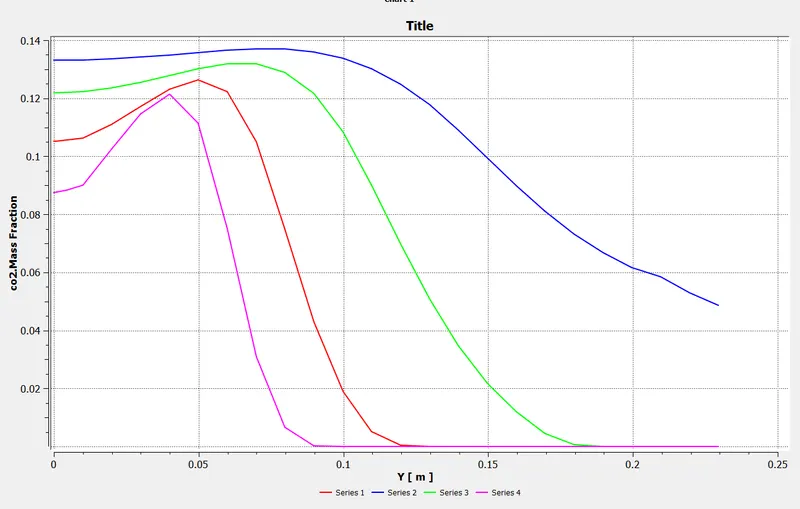
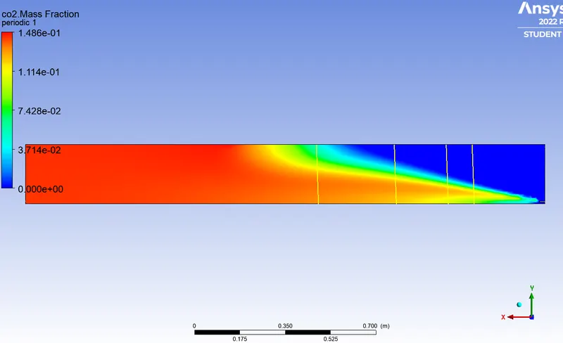
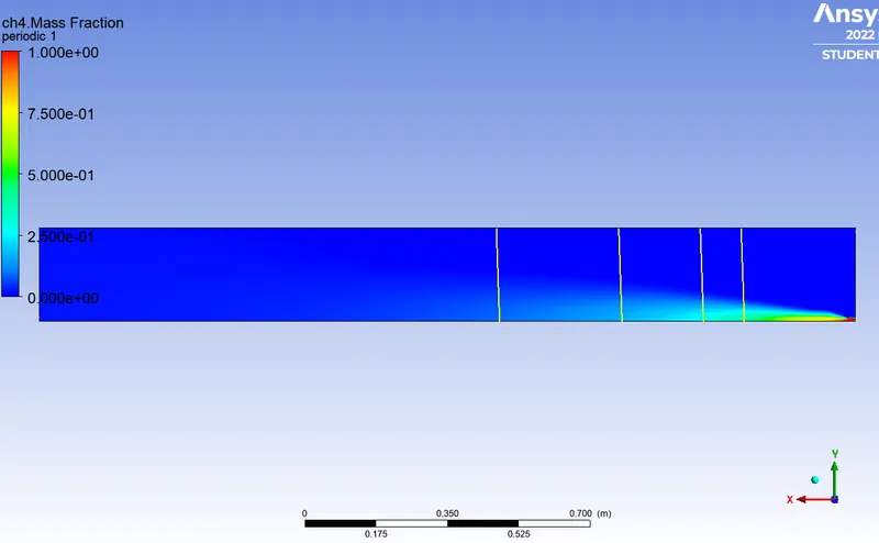
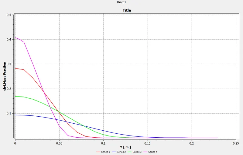
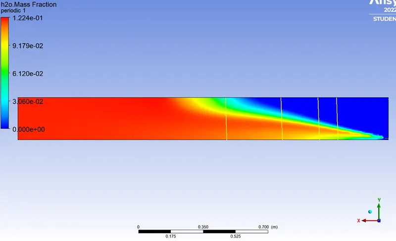
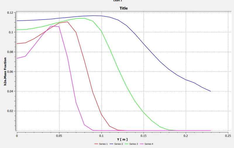
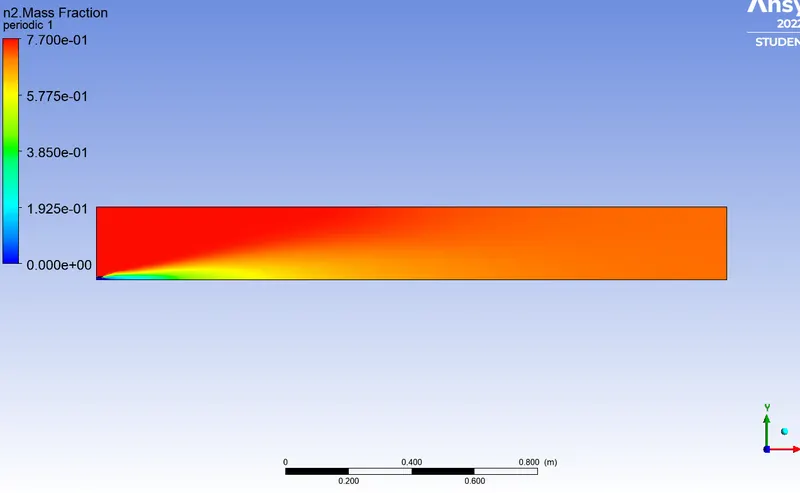
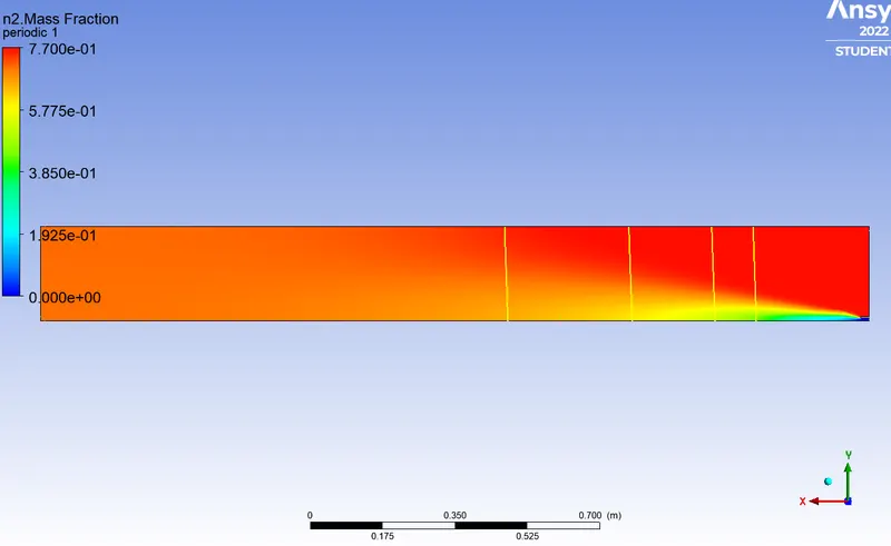
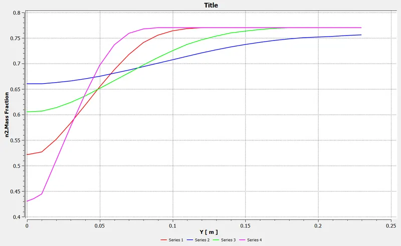
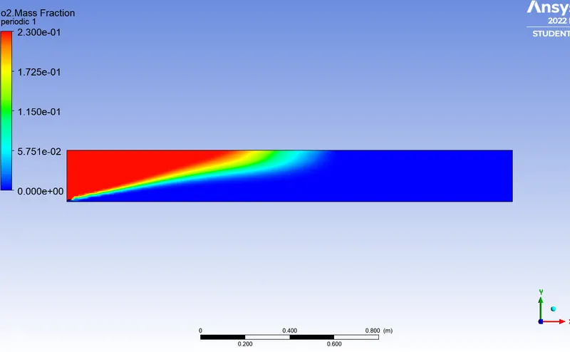
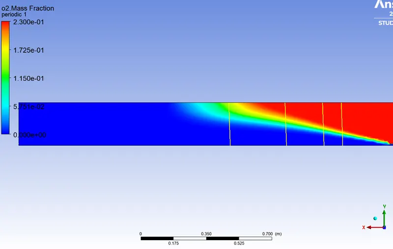
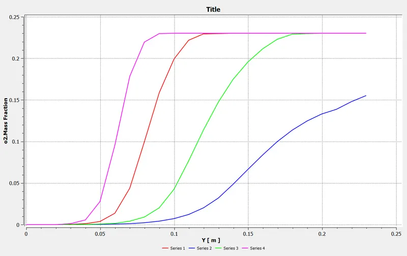
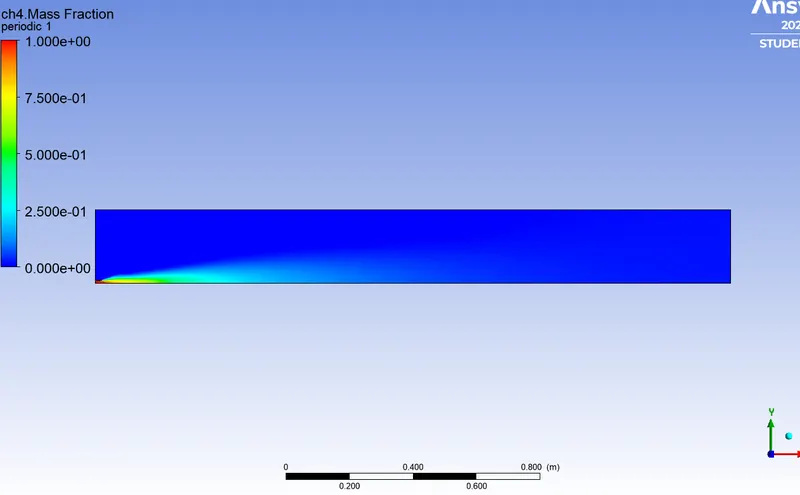
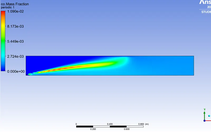
Perform a combustion simulation on the combustor model and plot the variation of the mass fraction of the different species’ in the simulation using line probes at different locations of the combustor as shown in Fig. You need to plot for CO2, H2O, CH4, N2, O2, NOx emissions & Soot formation.

Part II

As you must have observed from the above simulation, the Nox and soot is getting formed at the outlet of the combustor. Such formation has harmful effects on the environment and humans. The stringent government norms also demand the least formation of Nox and soot and to satisfy those requirements, you need to check the effect of adding the water in the fuel.

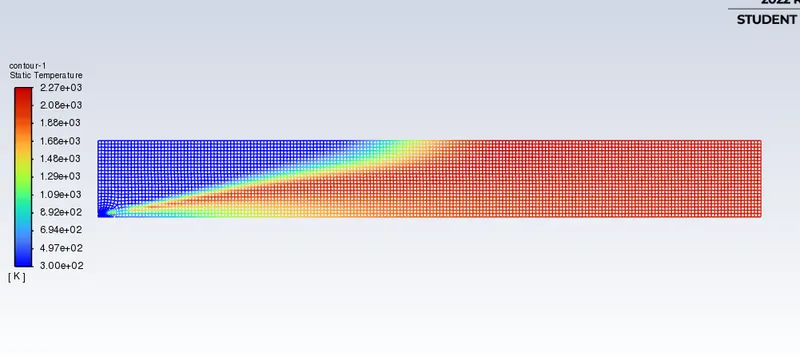
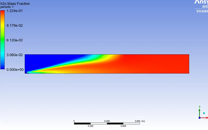
In this part, you need to add the water content in the fuel from 5% to 30% by mole and observe the effect of it on the results. It is necessary to provide line plots and contours to prove your claim.

You can use the parametric study approach if required.

Theory:

Chemical reaction models transform physical knowledge into a mathematical formulation that can be utilized in computational simulation of practical problems in chemical engineering. Computer simulation provides the flexibility to study chemical processes under a wide range of conditions. Modeling of a chemical reaction involves solving conservation equations describing convection, diffusion, and reaction source for each component species

Introduction:

The reaction rate or rate of reaction is the speed at which a chemical reaction takes place, defined as proportional to the increase in the concentration of a product per unit time and to the decrease in the concentration of a reactant per unit time. Reaction rates can vary dramatically. For example, the oxidative rusting of iron under Earth's atmosphere is a slow reaction that can take many years, but the combustion of cellulose in a fire is a reaction that takes place in fractions of a second. For most reactions, the rate decreases as the reaction proceeds. A reaction's rate can be determined by measuring the changes in concentration over time.

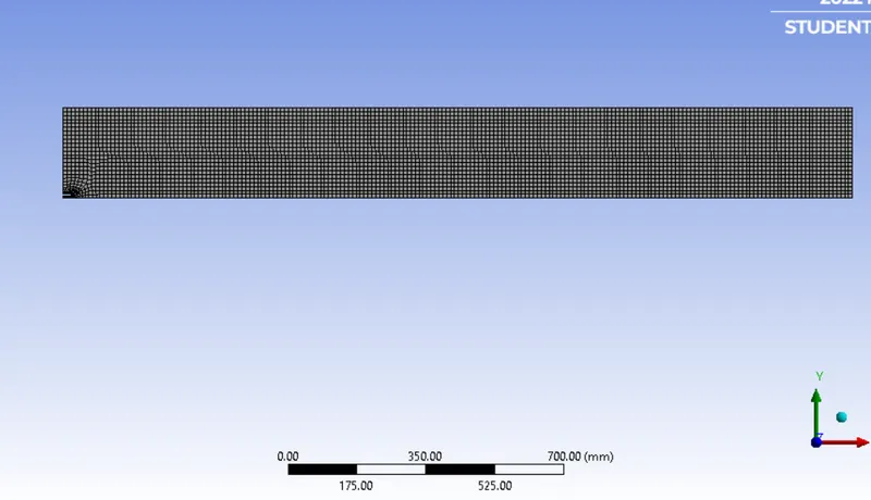
The eddy case consists of the flow modeling of reacting flow with an eddy-dissipation model such as k-ε. Here, ANSYS Fluent has used the k-ε model along with an implicit solver. It has been reported in [2] that this simulation was attempted with 417,000 cells and all-structured mesh. The benchmark results are shown in Figure 6.3. Three machines and their different configurations were used, including the famous hardware of Bull, Fujitsu, and IBM. For the Bull machine, the model was B710 with an Intel E5-2680 processor with a speed of 2.8 GHz with turbo-boost on, and the operating system was Redhat 6 with connectivity of FDR Infiniband by Mellanox. Two models of Fujitsu were tested, each with a difference in CPU speed of 2.7 and 3 GHz, respectively. IBM machines also differ in CPU rating; one is IBM DX 360 M3 with a 2.6 GHz processor and the other is IBM DX360 M4 with a 2.7 GHz processor. All used the same operating system, Redhat Linux 6, and FDR Infiniband of Mellanox for connectivity.

Geometry:

Model and simulation:

Meshing:

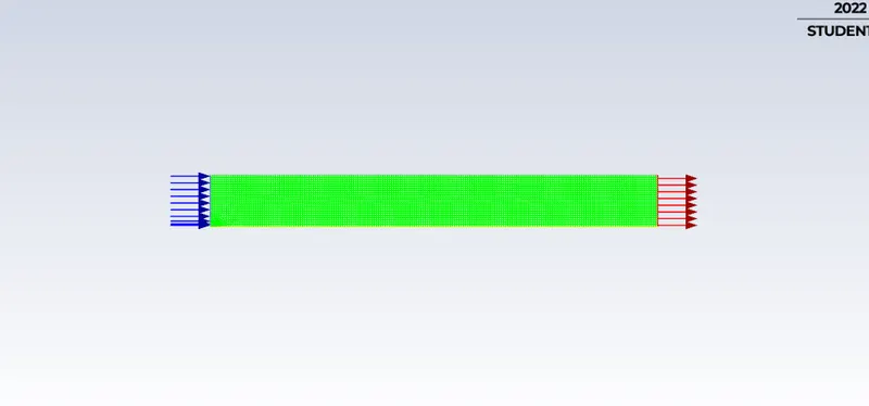
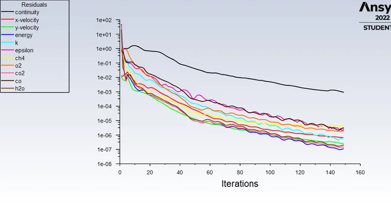
Setup:

Results:

Conclusion: