Week - 10 Hyperelastic Material Models

Aim : To simulate a tensile test by calculating the Mooney Rivlin and Ogden material constants and compare the both using stress-strain data from a Dogbone specimen tensile test with 100 percent strain.

Explanation :

Mooney Rivlin and Ogden material models are used to represent the hyperelastic materials. Hyperelastic materials are those material which have huge strain for small amount of stress and have Poisson’s ratio more than 0.49.

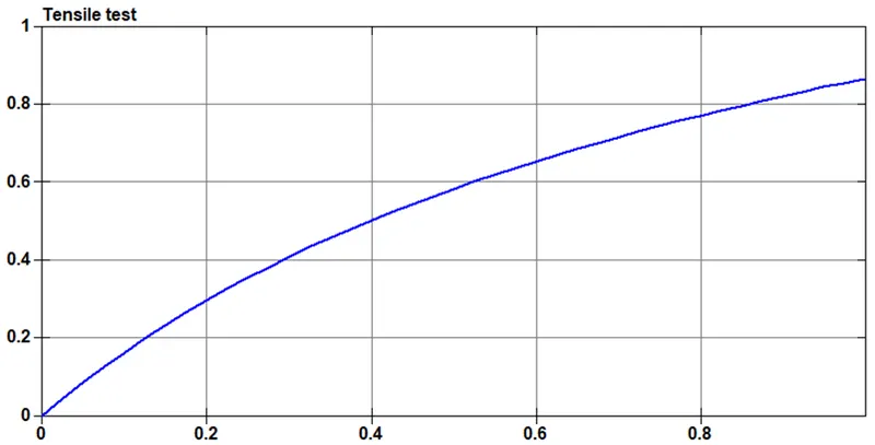
To calculate the Mooney Rivlin and Ogden material constants from LS Dyna, the engineering stress strain curve is used as input.

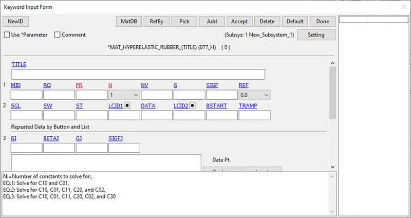
077_H_MAT_HYPERELASTIC_RUBBER

This material model provides a general hyperelastic rubber model combined optionally with linear viscoelasticity.

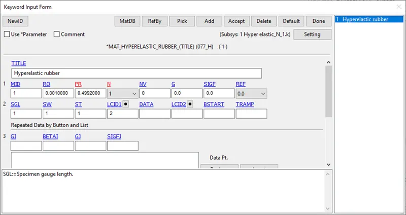
To calculate the Mooney Rivlin constants, the order(N) is toggled to either 1,2 or 3 and additionally, a load curve is loaded representing engineering stress vs strain. The values of SGL, SW, ST are toggled to 1.

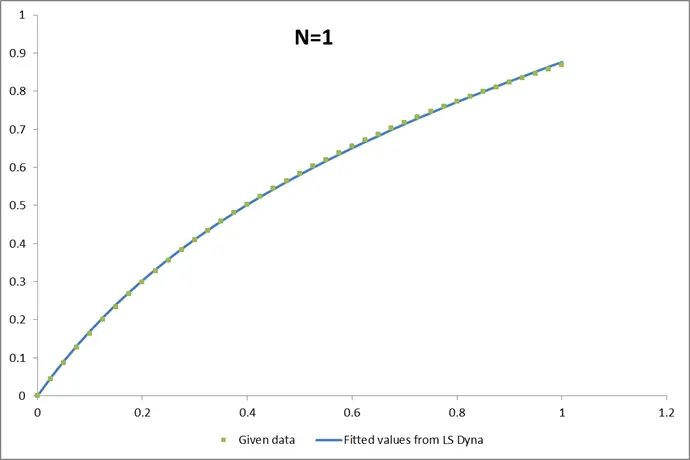
The constants for N=1 as reported from d3hsp file are

N=1

Mooney constant c1 =    0.1768, Mooney constant c2 =    0.1474

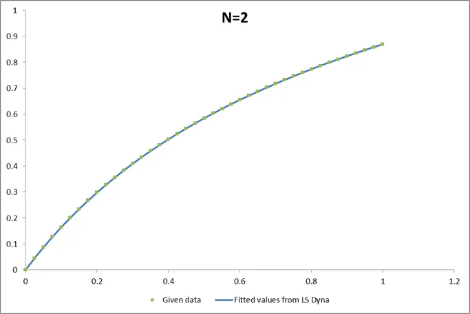
N=2

Hyperelastic Constant C10=    0.2595

Hyperelastic Constant C01=    0.04594

Hyperelastic Constant C11=   -0.02092

Hyperelastic Constant C20=    0.002914

Hyperelastic Constant C02=    0.001016

Hyperelastic Constant C30=    0.0000

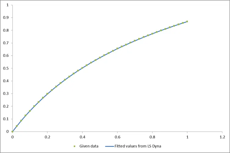
N=3

Hyperelastic Constant C10=    0.2611

Hyperelastic Constant C01=    0.04420

Hyperelastic Constant C11=   -0.006074

Hyperelastic Constant C20=   -0.002667

Hyperelastic Constant C02=   -0.009968

Hyperelastic Constant C30=    0.0001565

 

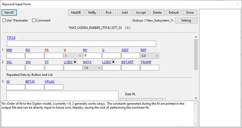
077_O-OGDEN_RUBBER

This material model provides the Ogden [1984] rubber model combined optionally with linear viscoelasticity.

To determine, the constants order(N) of the equation is entered and SGL,SW,ST is toggled to 1 and given load curve of engineering stress vs strain is loaded as curve in LS Dyna.

 

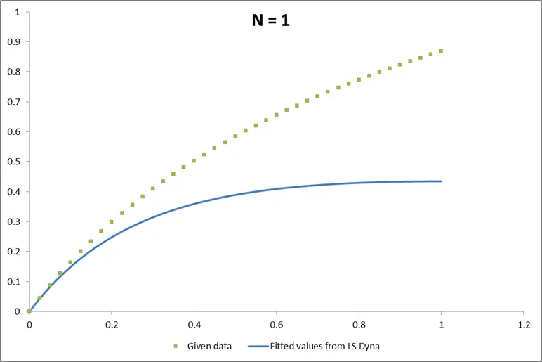
N=1

mu(1)= 0.910760  alpha(1)= 1.342723

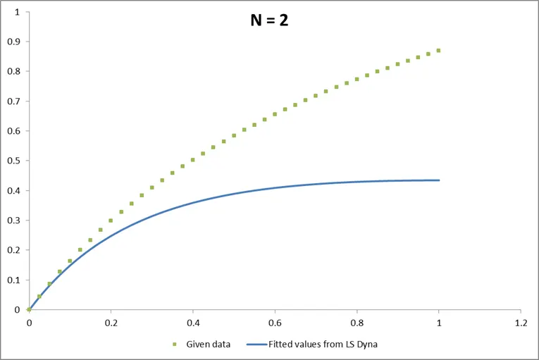
N=2

mu(1)= 0.915647  alpha(1)= 1.339909

mu(2)= 2.225955  alpha(2)=-0.001843

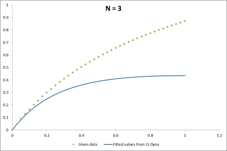
N = 3

mu(1)= -0.031842  alpha(1)= 1.926332

mu(2)=  0.261375  alpha(2)= 1.550340

mu(3)=  0.681991  alpha(3)= 1.288782

 

Comparing the various order fits of the two models, Hyperelastic model is able to capture all the features of the material than the ogden rubber. Further, using these constants, the dogbone case is setup. The stress strain values are compared against the different fits of two material model.

PRE-PROCESSING : 

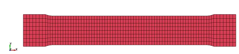
(1) Modelling/ Discretization : 

The input file consists of a dogbone specimen.

(2) Section properties : 

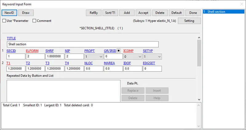
The element formulation elform=2 (default element type), is used with thickness specified as 1.2 mm.

(3) Material properties : 

A material keyword is defined either by including the constants as calculated by LS Dyna shown in the earlier steps or defining the Engg stress vs strain curve by denoting the order of fit (N=1 in this case). The given load is defined by loading the XY data.

(3) Boundary conditions/Constraints/Loads: 

Boundary conditions:

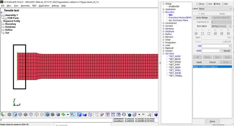
To simulate the fixed end, one side of the nodes are constrained in the axial direction (along x direction).

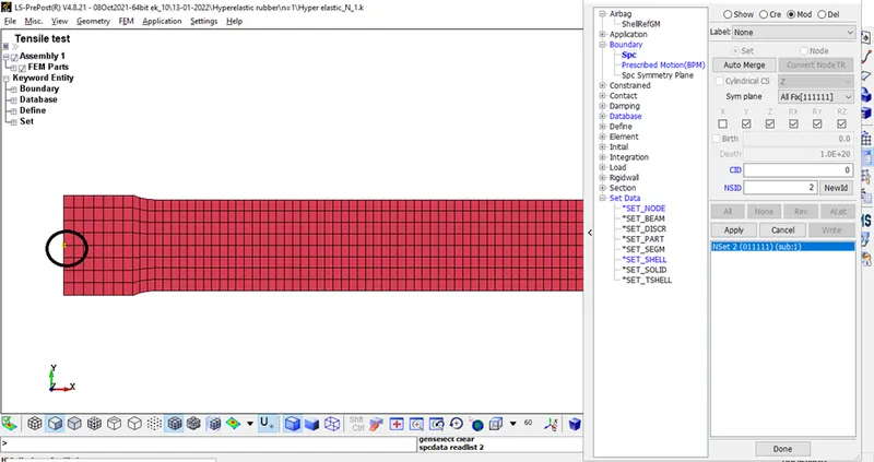
Another SPC is created to constraint the mid node along lateral direction to allow nodes above and below it to move along this direction (y direction).

Load: 

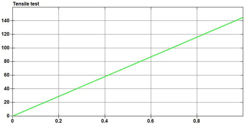
A load curve is created to define the load vs displacement curve to apply the prescribed strain(100%). Since the length of the specimen is 145 mm, a load of 145 mm is applied in 1 step.

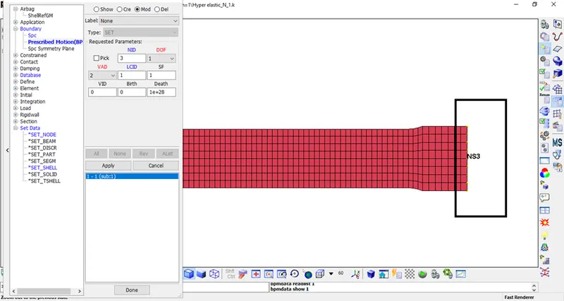
A PRESCRIBED_MOTION_SET is defined on the other end of the specimen to apply the load.

(5) Control :

Implicit general:

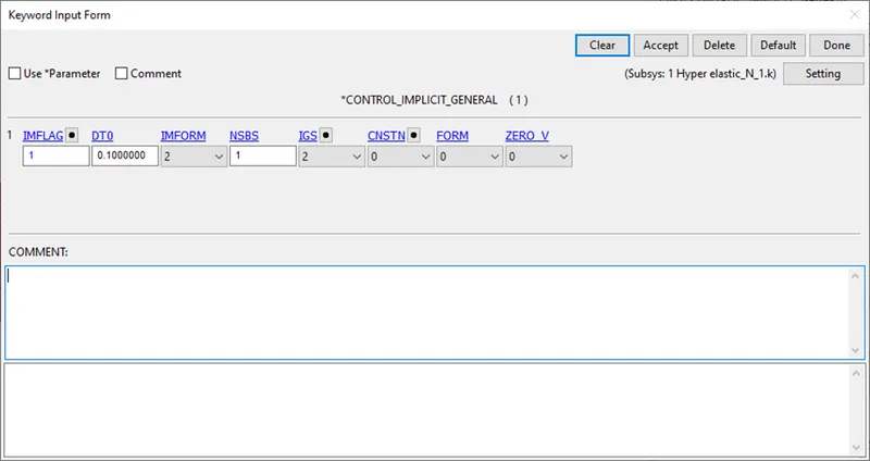
As tensile test is a steady state test, we run an implicit analysis. To activate implicit analysis Control_Implicit_General keyword is to be added. IMFLAG = 1 activates the implicit analysis. DT0 is initial time step that is defined as 0.1

Implicit auto:

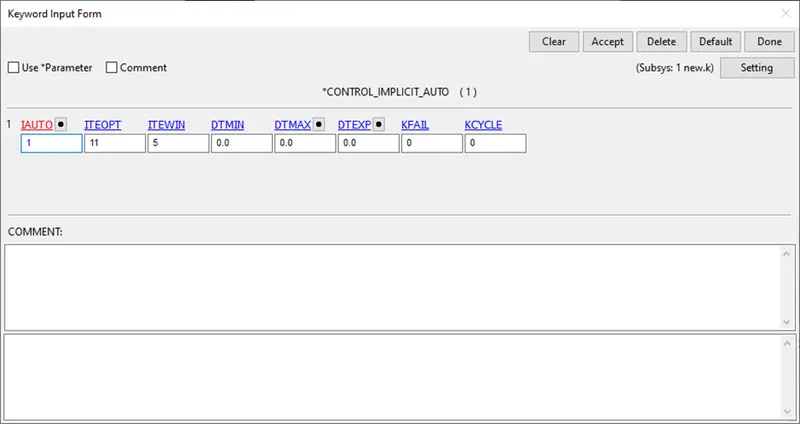
Implicit auto used to fine tune the solver. IAUTO is used to automatically adjust time step size in order to lessen the number of load increments. ITEOPT and ITEWIN are used to either increase or decrease the load increments. These have to be cautiously selected so as to run the solution in unreliable or expensive condition.

Implicit solution:

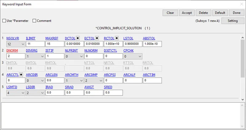
NSOLVER is used to select the solution method for implicit analysis. Since the material is non linear, Nonlinear with BFGS updates + optional arclength solver (NSOLVER =12) can be used with rest of parameters left default.

Implicit solver:

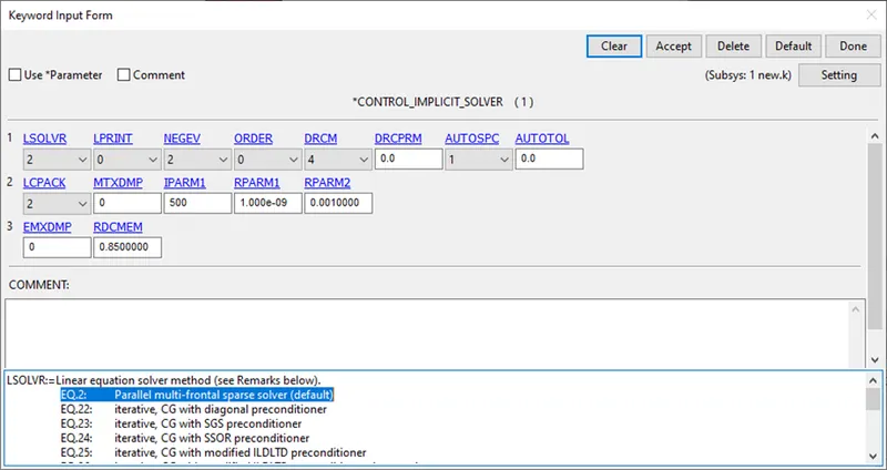
Implicit solver is used to invert the stiffness matrix in each iteration to check for residuals. The default Parallel multi-frontal sparse solver is used with LCPACK library.

Termination:

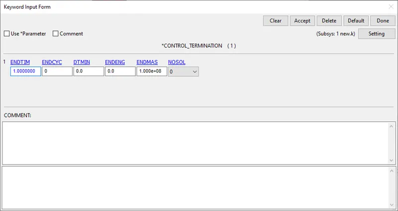
Since the load is applied in 1 step, control termination keyword is used to denote the end time as 1.

(6) Database :

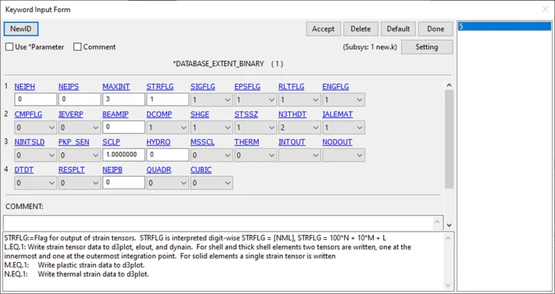
Binary D3Plot is written for every 0.1 unit interval of time. Extent binary is used to derive strain tensor data by denoting STRFLAG as 1.

(7) Part :

In this section, the different parts/components in the file are connected to their respective material ID and section ID.

Once all the above is done, Model check is done to ensure all the parts are connected to their respective material, section are all well defined.  A dialog box containing the cards - the errors, warnings, unreferenced, undefined are displayed. Approppriate action should be taken to overcome errors and warnings can be minimised.

SOLVING :

The above created input file is saved as keyword file (.k extension). This keyword file is solved using LS DYNA manager.

POST PROCESSING :

Various contour plots are plotted to check for sanity of the problem being solved. The animated file of the problem can be checked by running the d3plot file in the LS-PrePost.

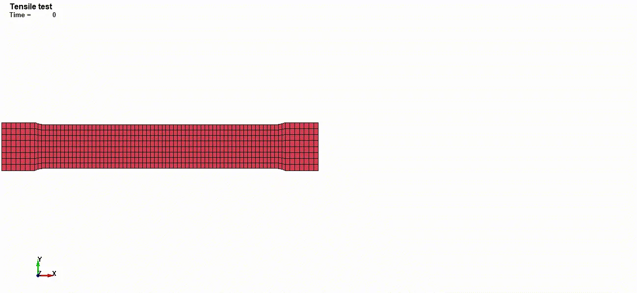
Animation of the tensile test

Stress, strain plots:

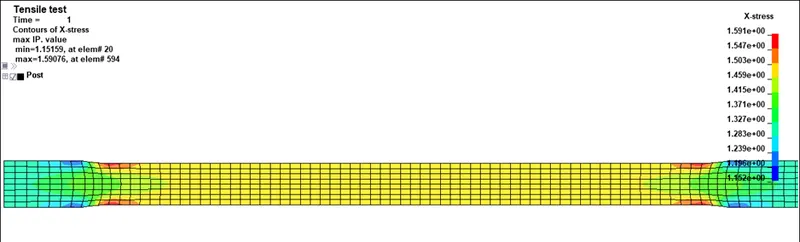
Directional stress(x direction)

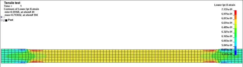
Directional strain(x direction)

Comparison of different fits of the two material models:

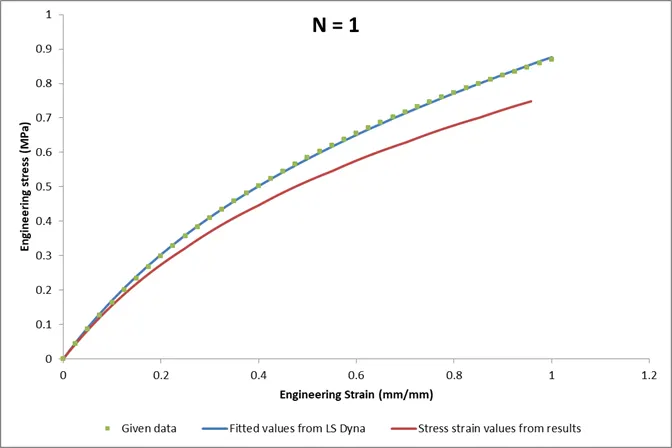
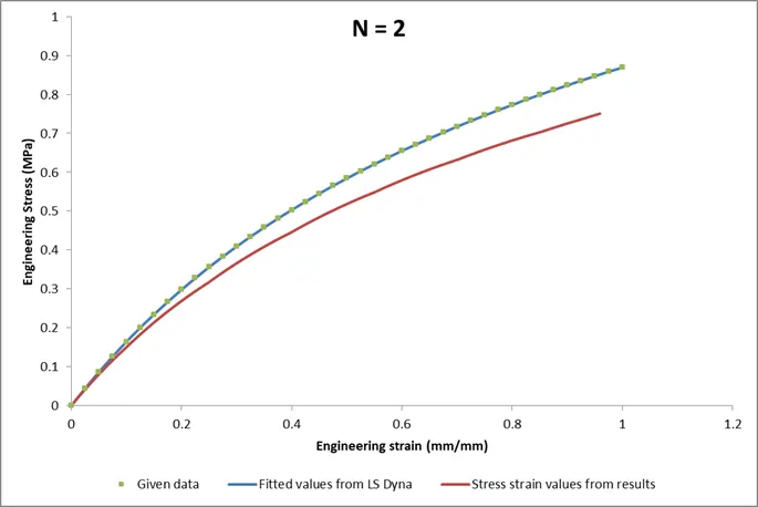
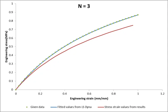
Hyperelastic Rubber

  

Ogden rubber

   

 

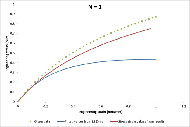
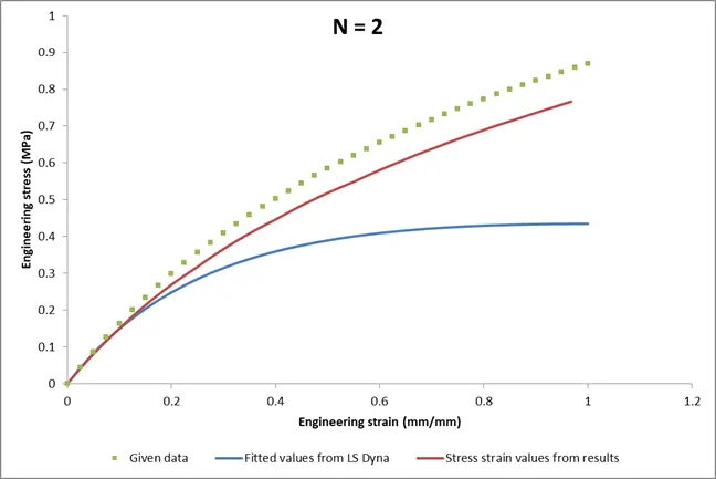
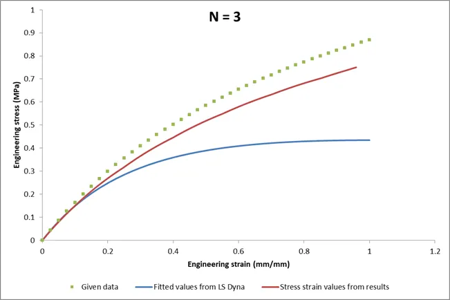
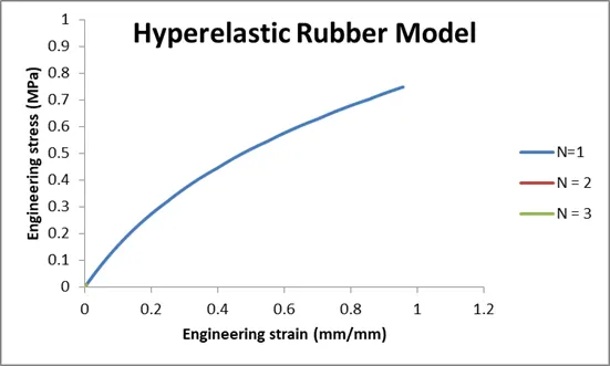
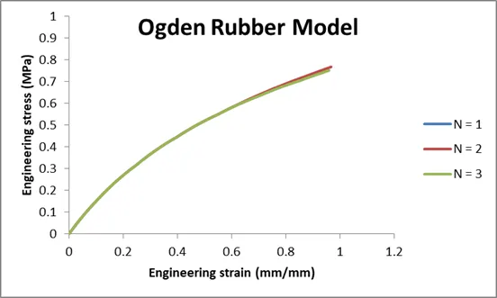
Comparison of stress vs strain curve of reported values of different order for Hyperelastic and Ogden rubber model 

From the above plots, we can infer that Hyperelastic rubber model is better at capturing the features of the material compared to Ogden model. Though there is no much change in values of stress and strain as extracted from simulation test because of small coefficients of higher order models both in Hyperelastic rubber model and Ogden models.

Conclusion:

Material constants were determined using Hyperelastic rubber and Ogden models of various orders (N=1,2,3). The different models were compared and the Hyperelastic model was found to be a better fit.

Tensile tests were run for the two material models of all the orders. The stress and strain values were compared and the values did not vary much.

Please follow the link to access the input, output files: https://drive.google.com/drive/folders/13h5nlD5I_HtAHbDKwuAPB-RxjW8pSKy9?usp=sharing