Challenge

Week - 10 Hyperelastic Material Models

AAsad K P31 Jan 2025

Week - 10 Hyperplastic Material Models

Aim

Determine the Mooney-Rivlin and Ogden material constants from the given engineering stress-strain data of a Dog bone specimen tensile test at 100% strain. Following the calculation, the two models will be compared using the stress-strain data, visualized through the analysis of the '.d3hsp' file and simulations.

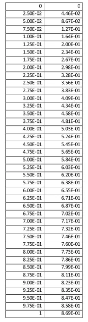
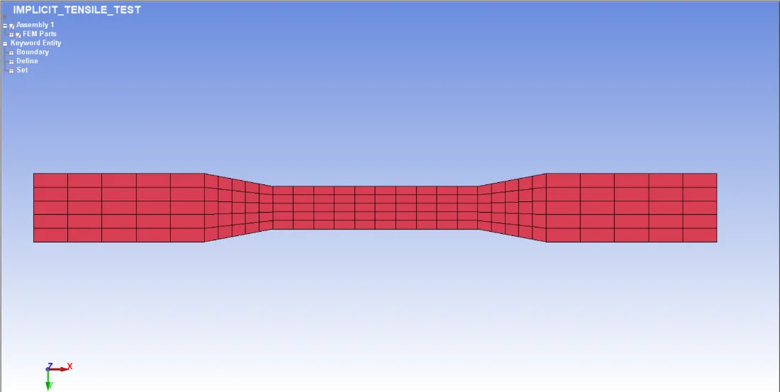
Output Required

Procedure

Step 01: Plotting given engineering stress-strain data

Initially, we must tabulate the engineering stress and strain data using Excel software. The given stress is in MPa and mm/mm units. Then plot a chart with engineering strain at the X-axis and engineering stress on the Y-axis.

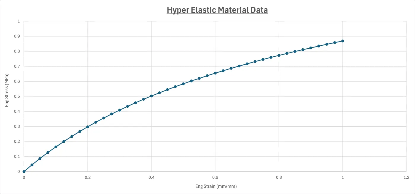
Step 02: Define the curve for the model using the provided data.

Open the keyword file in Notepad++. Using the provided data, define a curve card for the model in Notepad++. Save the file to the preferred location. Open LS Prepost and load the newly modified keyword file. Then, open the curve card, plot the curve data, and compare it to the actual graph obtained earlier from the Excel file.

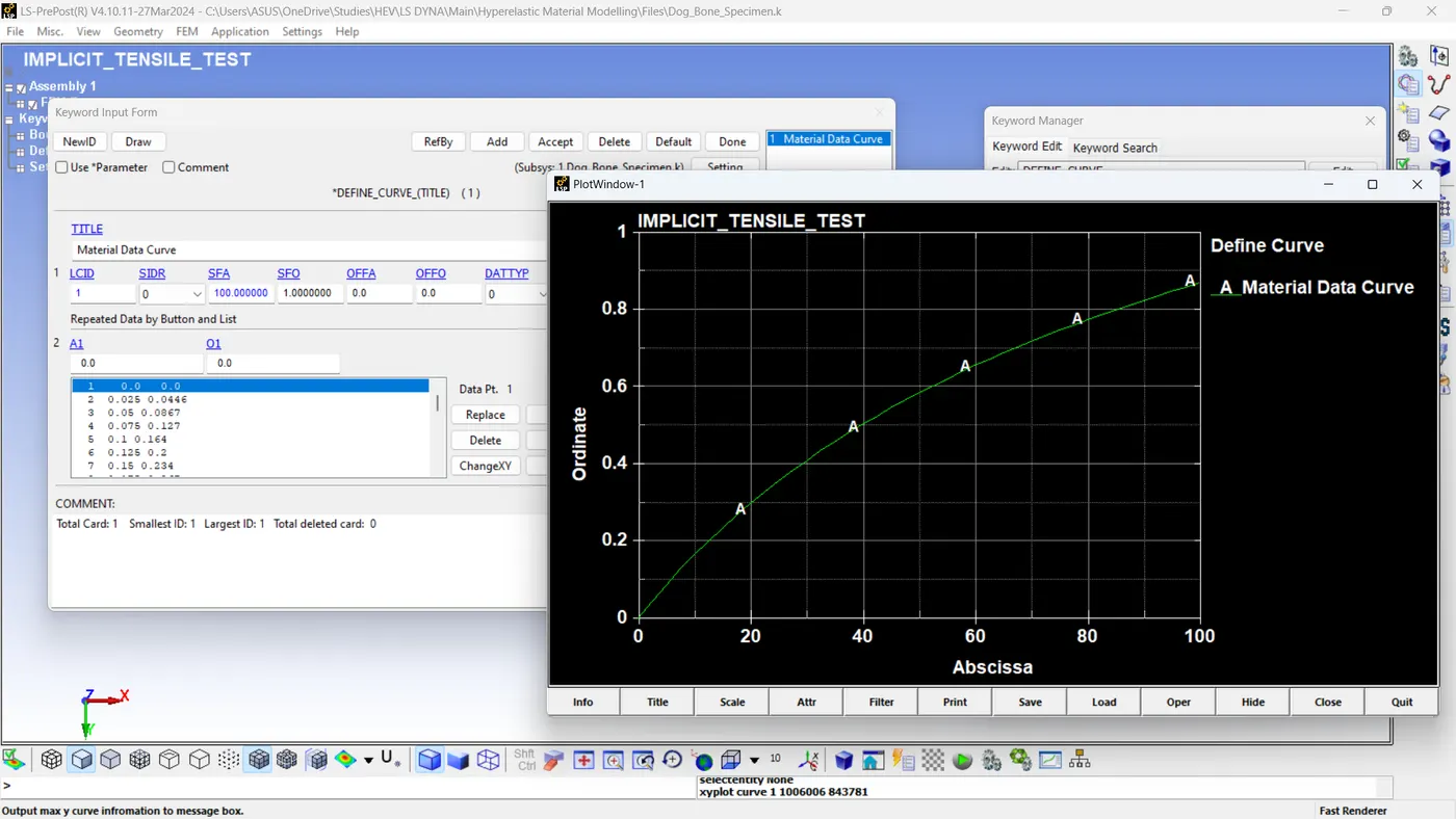
Step 03: Material Definition

Our goal is to define the model using hyperelastic material. We use MAT 077_H HYPERELASTIC_RUBBER and MAT 077_O OGDEN_RUBBER material cards. Run the simulation using these cards separately with different files.

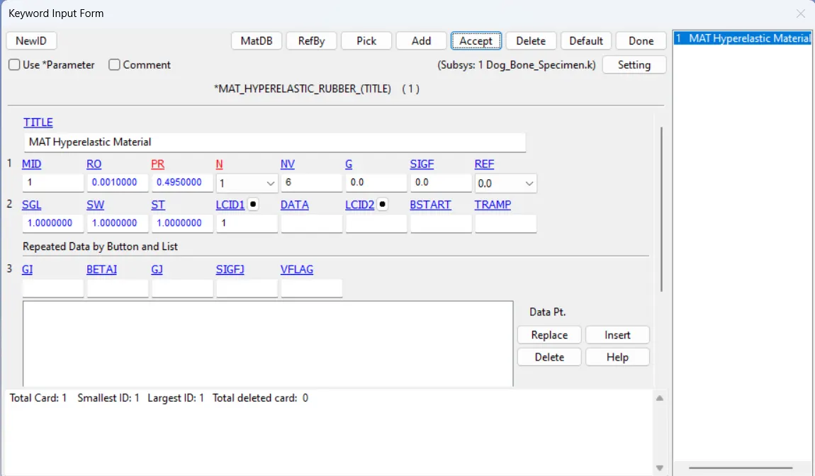
1. MAT 077_H HYPERELASTIC_RUBBER

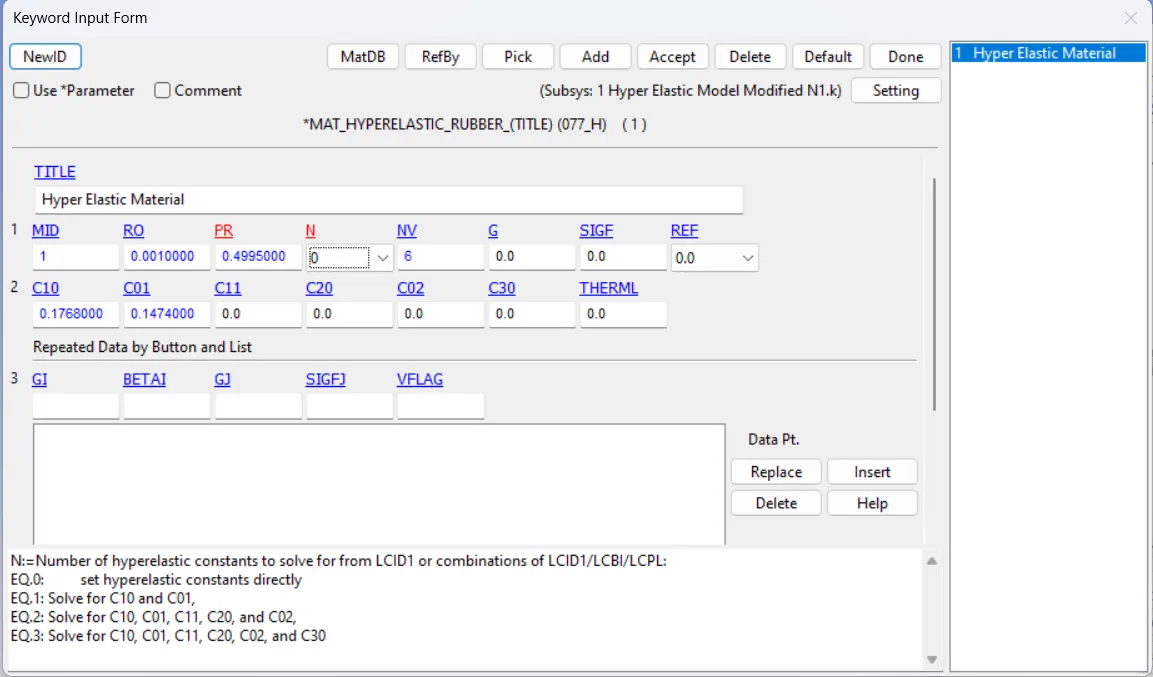
For the initial simulation, we aim to determine the values of C01 and C10. By setting N = 1, we will execute the simulation to ascertain the values of C01 and C10. Additionally, the LCID is defined by the curve derived from the provided material data. Other parameters will be

RO = 0.001 g/mm³

PR = 0.495

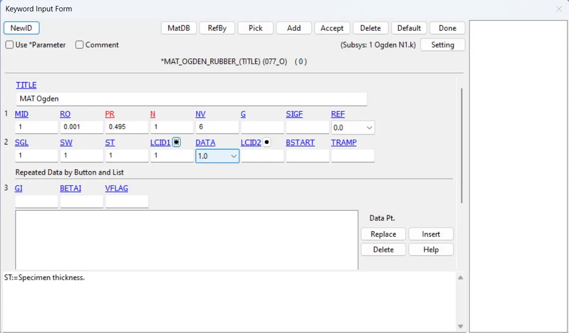
2. MAT 077_O OGDEN_RUBBER

Here, instead of C01 and C10, we need to find the values of µ1 and α1. We will execute the simulation by setting N = 1 to ascertain the values of µ1 and α1. Additionally, the LCID is defined by the curve derived from the provided material data. Other parameters will be

RO = 0.001 g/mm³

PR = 0.495

Step 04: Assigning Boundary Conditions

For every model, we need to define a boundary condition that reflects the tensile test of the given specimen. For that first, we need to define the required Node Sets.

Node Set 1 = For restricting motion in the left end.

Node Set 2 = For the tensile motion in the right end

Node Set 3 = For the restricting motion in the neutral axis.

For Node Set 1 and 3, we can use SPC_Node Set cards and control the motions by constraining specific translational and rotational DOFs. For Node Set 2, we can use a Prescribed Motion card, and it can be defined by displacement curve.

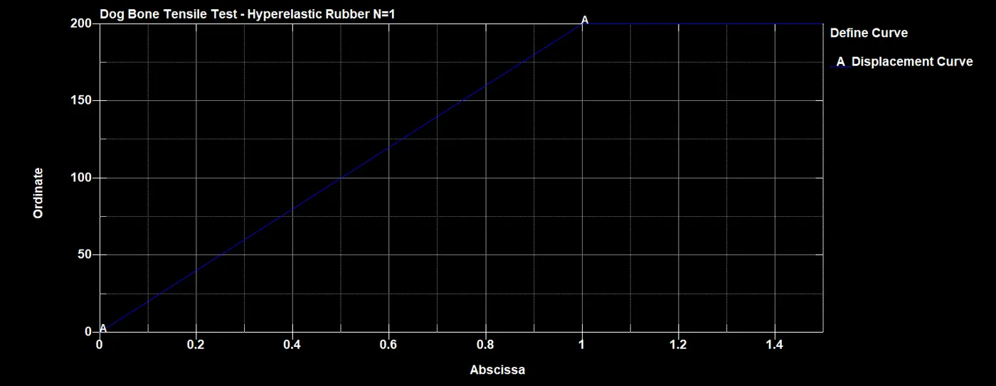
From the objective, the tensile test is carried out by a strain of 100%. That means the change in length after the tensile test is equal to the original length. By measuring the model, we can see that the specimen length along the x-axis is 200mm. This means the change in length after the tensile test should be 200mm.

The curve is defined to represent the tensile motion. Using the curve, we can assign a prescribed motion to the specific node sets.

Step 05: Section and Part Definition

For each model, the section will be defined using ELFORM=2. Then, the part will be assigned using the defined material and section cards.

For each model, the section will define using ELFORM=2. Subsequently, the part is assigned by the defined material cards.

The database includes the following cards defined for its outputs.

1. ASCII Option Database includes GLSTAT and MATSUM with DT = 0.1
2. BINARY_D3PLOT Database with DT = 0.1
3. EXTENT_BINARY Database with STRFLG = 1

It is an implicit analysis, so define the control cards according to it. The following control cards should be assigned to the model.

1. IMPLICIT_AUTO
2. IMPLICIT_GENERAL
3. IMPLICIT_SOLVER
4. IMPLICIT_SOLUTION
5. CONTROL_TERMINATION

Step 06: Initiating First Simulation and Finding the Constants

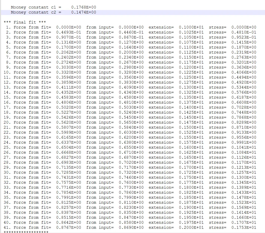
After the model definitions, we need to save the file to a specific folder with a specific file name. Then run the implicit simulation. After the normal termination of the simulation, open Notepad++ and open the D3HSP file. Then search the keyword C1 and find the values of constants. The value of C1 represents C10 and C2 to the C01. Also, we can see the extension and true stress of the simulation.

And from the simulation,

C1 = C10 = 0.1768
C2 = C01 = 0.1474

Also, we can see the extension and true stress values of the model. From this, we can calculate the engineering stress and engineering strain values. Using the below equations,

Engineering Strain, Σ_e= λ - 1
Where λ = Stretch /
Engineering Stress, σ_e = Σe/λ

Step 07: Modifying the Material Data Using the Constants

Open the MAT 077_H material card and change N=0. Then update the values of C10 and C01 and save the model in a separate location with a suitable name.

Step 08: Simulation and Results

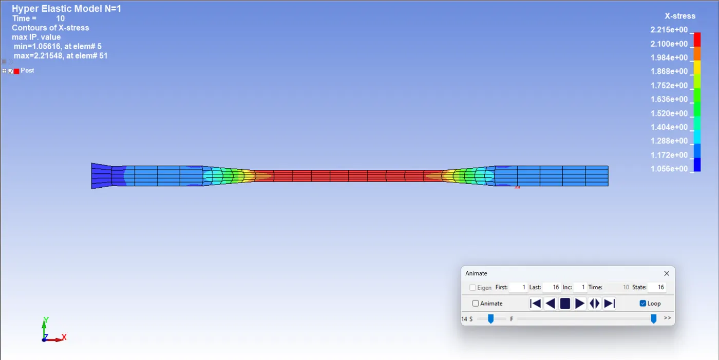
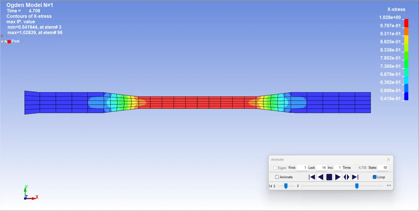
Simulate the model with the updated material card. Analyse the D3PLOT animations and D3HSP file and table out the desired values.

Step 09: Repeating the Process for Different Cases

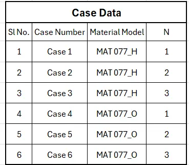
We aim to repeat the procedure by changing the N value from 1 to 3. The material card will be MAT 077_H and for each case, we need to find out the Mooney-Rivlin material constants for the material model. Then for every case, we need to change the N value to 0. Put the corresponding Mooney-Rivlin material constants and analyse the results. Tabulate the stretch and true stress values, find out the engineering stress and strain values and plot the graph between them. Compare the given plots and study the results for each value of N.

Similarly, we need to change the material model to the MAT 077_O Ogden model. Here we need to find out Ogden material constants for the values of N from 1 to 3. Then, repeat the process and analyse the results.