Hyperelastic Material Modelling

AIM:

Material modeling of MAT- 077_H, 077_0, Hyperelastic Rubber, and Ogden Rubber card from raw data and fit the experimental values to the raw data by Curve

OBJECTIVE :

1. Extract the Engineering Stress/strain data from the given image.

2. Convert the data into the required SI unit by calculation. here the unit system taken is gm-mm-ms, GPA.

3. Plot the data as a curve to define in the material card.

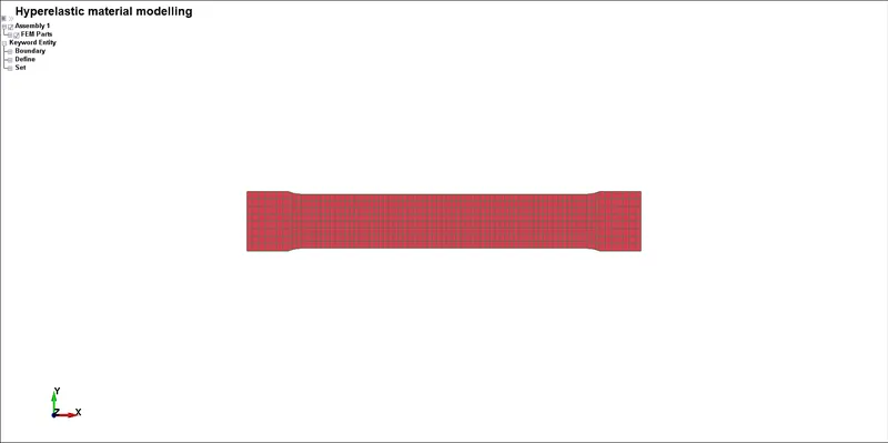
4. Setup the simulation for the tensile test on dogbone specimen to get the results.

5. validate the output data by checking that it matches with the original data.

Hyperelastic Materials:-

• A hyperelastic or Green elastic material is a type of constitutive model for ideally elastic material for which the stress–strain relationship derives from a strain energy density function. The hyperelastic material is a special case of a Cauchy elastic material

• They are highly elastic materials so that their deformations can be recovered when subjected to very large strains.
• For many materials, linear elastic models do not accurately describe the observed material behavior.
• The most common example of this kind of material is rubber, whose stress-strain relationship can be defined as non-linearly elastic, isotropic, incompressible, and generally independent of strain rate.

In contrast, hyperelastic materials are described through a strain-energy density function. The strain-energy density can be used to derive a nonlinear constitutive model (i.e., stresses as a function of large strain deformation measures like deformation) which are derived by researches and some acceptable models we are using popularly such as Neo-Hookean, Mooney-Rivlin, and Signorini models, Ogden, Yeoh, Arruda-Boyce.

Mooney Rivlin:

The strain energy density function for an incompressible Mooney–Rivlin material is defined as

Where Cij">Cij are empirically determined material constants, I1 and I2 are the first and the second invariant. By varying the Index values of I and j we can change the constitutive equations and use them appropriately for our component. Similarly, we will be having multiple coefficients C. This changing of the index will be basically changing the order of the polynomial of the energy density equation. We need to find out the coefficients of these material models for a different order of the polynomial and extract the best fit curve data from the D3HSp file and compare it with the material curve.

Ogden Material:

The Ogden material model is a hyperelastic material model used to describe the non-linear stress–strain behavior of complex materials such as rubbers, polymers, and biological tissue. The model was developed by Raymond Ogden in 1972. The Ogden model, like other hyperelastic material models, assumes that the material behavior can be described by means of a strain energy density function, from which the stress–strain relationships can be derived.

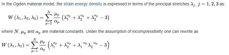
In our case, we will be validating the experimental data, provided for a hyperelastic material subjected to a uniaxial tensile test, with LS-DYNA simulation data using Mooney-Rivlin and Ogden material models.

PROCEDURE :

1. Lab test data Image is provided where the data points should be Exported to Excel Sheet

2.The Data given is in Engineering stress/Strain

3.Eng stress vs Strain Value is plotted up to Strain rate of 100% which is 1

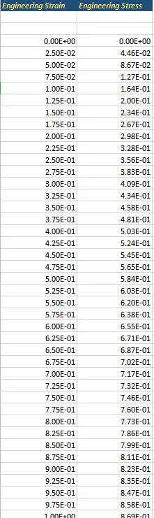
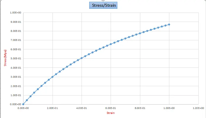
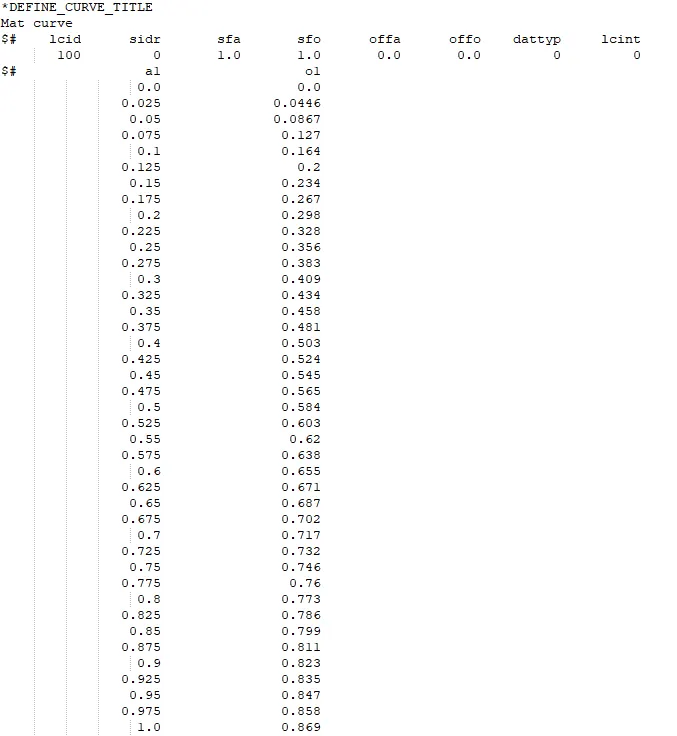
4. These Values are Taken into account and Inputted in Load curve LCID For Tensile Test using Dogbone Specimen In LS-Dyna

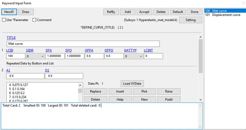
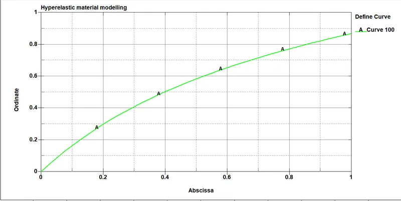
5. The Material Curve Is plotted using These Values

Section Creation:-

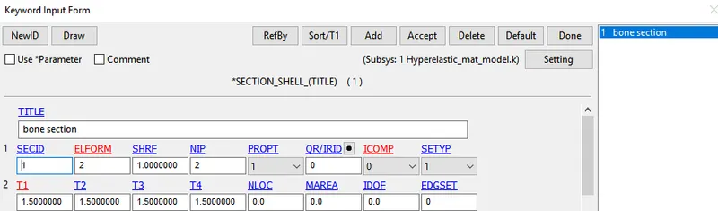
Section Shell is Assigned to the Dogbone Specimen with ELFORM=2, and Thickness is Assigned as 1.5mm.

Material:-

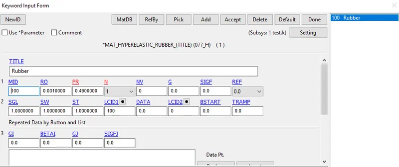
The material card is defined as the behavior of Hyper-Elastic material MAT- 077_H_ Hyperelastic Rubber is Assigned with Material Properties of Rubber

Density=0.001 gm/mm^3

Poissons Ratio=0.49

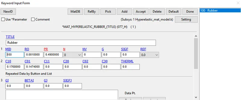
The N parameter in the *MAT77_H material card represents the order of polynomial for which the constants are required to solve. This involves N1, N2, and N3 cases where the constants are solved along with stretch and true stress data.

The Mooney-Rivlin constants for each polynomial order cases are:-

N1 Solves for Two Polynomials C10, C01

N2 Solves for Six Polynomials C10, C01, C11, C20, C02, C30

N3 Solves for Six Polynomials C10, C01, C11, C20, C02, C30

The SW, SGL, and ST parameters are set to unity as we have a stress-strain load curve unlike in the case of force-displacement data that requires specimen dimensions.

SW-Specimen Width

SGL-Specimen Gauge Length

ST-Specimen Thickness

The Model is Solved For N1, N2, and N3 Polynomials, and then the obtained values are Inputted according to the Constants In N0

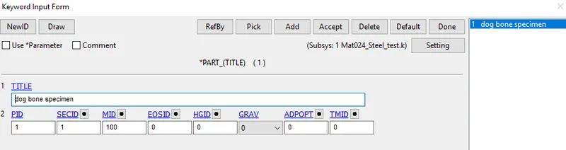
Assign the Section and Material To the Part

Boundary Conditions:-

Tensile testing, also known as tension testing is a fundamental material Science and engineering test in which a sample is subjected to a controlled tension until failure.

For the Process One end of the Specimen is Fixed and the Displacement is Given at another end

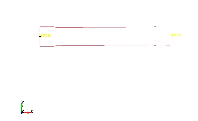
A set Of SPC nodes are Created at one end and Constrained at all Dof's

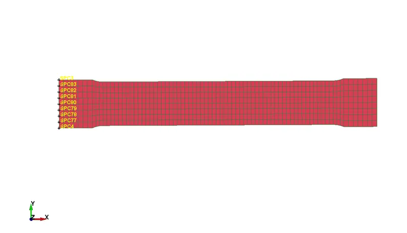
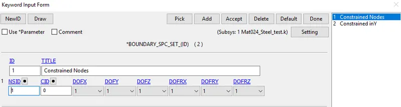
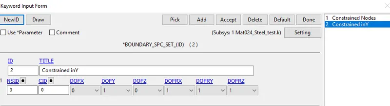
A Node in the Middle is selected from Both sides and Constrained In Y so that it cant Move From centre

Displacement:-

A set of nodes are selected from the Free end By using create entity > Set Node

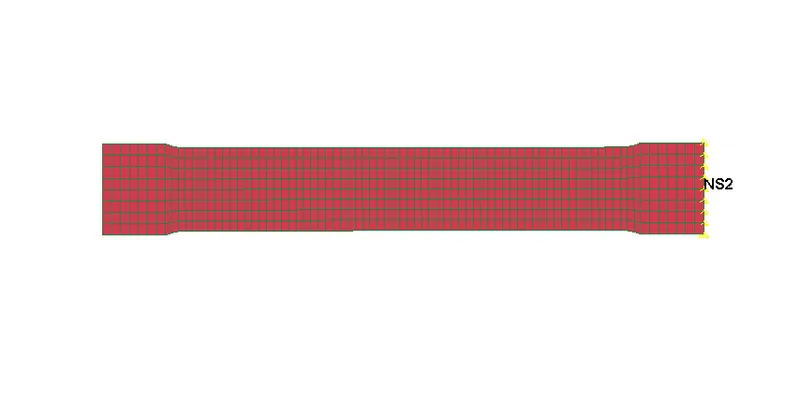
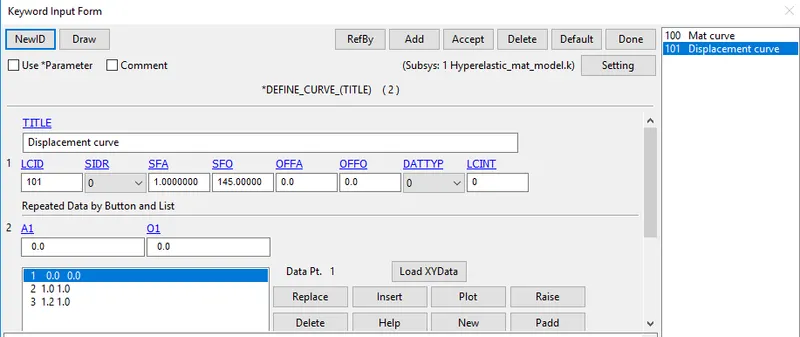
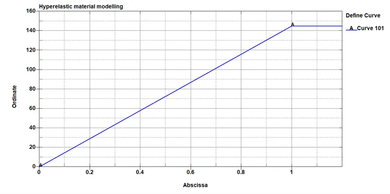
The Displacement Curve is defined Using Define > curve

as the Stretch Given Here is 100%

`epsilon=lambda-1`

`epsilon=2-1`

`epsilon=(Delta)/l=1`

L=145( length of the specimen)

Displacement ordinate is scaled as 145

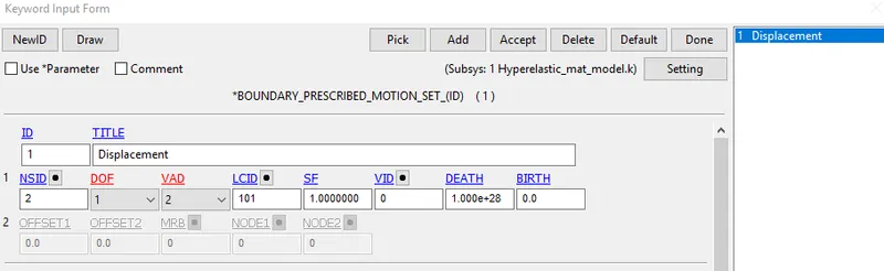
Boundary Prescribed Motion Set:-

The Displacement Curve is Assigned To the Node set By Boundary Prescribed Motion Set

Choose VAD=2 It refers to Displacement

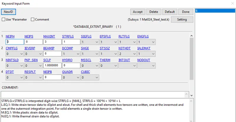
To Record, the Strain In order to Plot Effective Plastic Strain vs Effective Stress Database Extent Binary Plot is Created to record the Strain tensor Values While STRFLG is set to 1

For running The Static Structural Analysis Implicit Solver is Best, So Implicit is preferred here for Simulation

As the LS-Dyna is explicit software in General, Some Control cards must be defined For switching to Implicit

1.Control_implicit_Auto:-

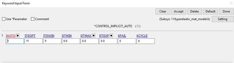
CONTROL_IMPLICIT_AUTO card is used for automatic time step control during implicit analysis. Input value for Automatic time step control flag = IAUTO = 1.

2.Control_Implicit_General:-

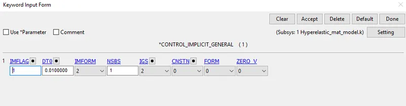
CONTROL_IMPLICIT_GENERAL card is used to activate implicit analysis and define associated control parameters. This keyword is required for all implicit analyses.

The input value for IMFLAG=Implicit/Explicit switching flag = 1 (implicit analysis)

DT0=Initial time step size for implicit analysis = 0.01

Control Termination:-

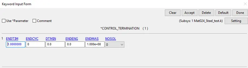
Control Termination Card is used to define the End Time of the Simulation

Output Requests:-

1. To view the results of Simulations Following Steps are Specified.

2.The time interval between the outputs is 0.1 is defined in D3plot

3. Go to Keyword Manager > Database > ASCII select GLSTAT, ELEOUT with DT 0.1

Analysis setup for Curve Fit:-

1.For N=1:

1. Save the Keyword and run the Model In Ls Dyna manager

2. Open the d3hsp File in Notepad++ for Mooney Rivlin COnstants

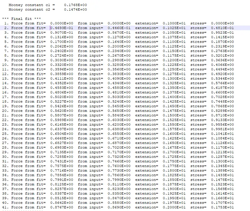
3. From The d3hsp file, Mooney Rivlin constants are obtained along with the Stretch and true stress values

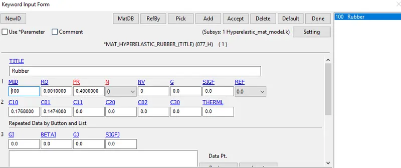
C10=0.1768E+00

C01=0.1474E+00

The stretch and True Stress values are converted into Engineering Strain and Engineering stress values

Stretch is Change in length by original Length which is denoted by `lambda`

Engineering Strain=`lambda-1`

Engineering Stress= True stress/1+Engineering Strain

2. For N=2:-

1. Change N=2 from the Material card and Run the simulation again

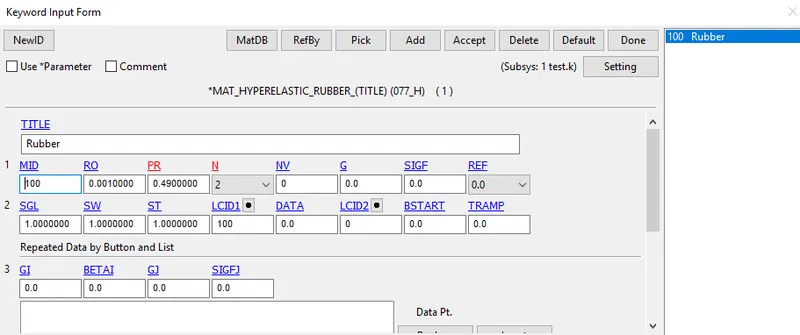
2. Open the d3hsp File in Notepad++ for Mooney Rivlin COnstants

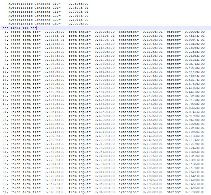
3. From The d3hsp file, Mooney Rivlin constants are obtained along with the Stretch and true stress values

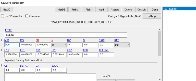
C10=0.2595000

C01=0.4594E-01

C11=-0.2092E-01

C20=0.2914E-02

C02=0.1016E-02

C30=0.0000E+00

Similarly, the Stretch and True stress values are converted to Engineering Strain and Engineering stress values

3.For N=3:-

Change N=3 from the Material card and Run the simulation again

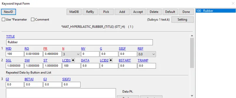
2. Open the d3hsp File in Notepad++ for Mooney Rivlin Constants

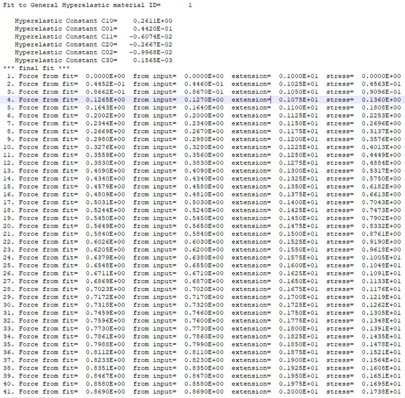
3. From The d3hsp file, Mooney Rivlin constants are obtained along with the Stretch and true stress values

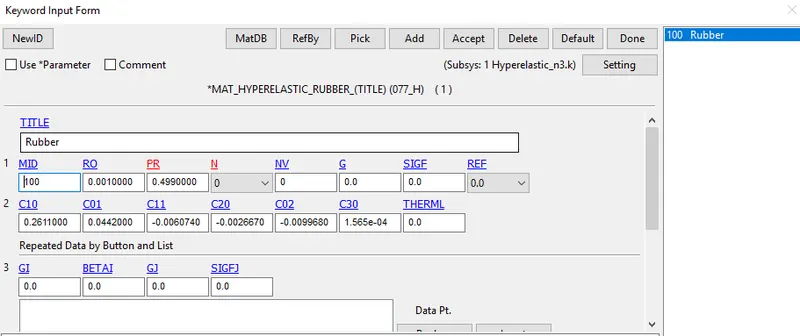
C10=0.2611E+00

C01=0.4420E-01

C11=-0.6074E-02

C20=-0.2667E-02

C02=-0.9968E-02

C30=0.1565E-03

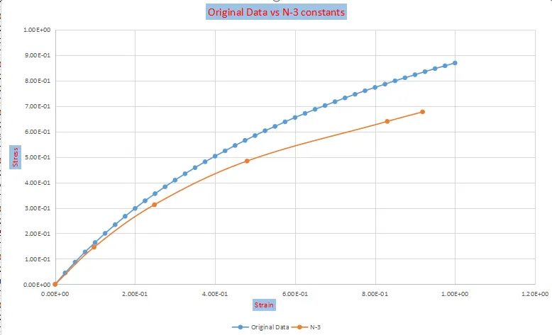
Similarly, the Stretch and True stress values are converted to Engineering Strain and Engineering stress values

Converted Values:-

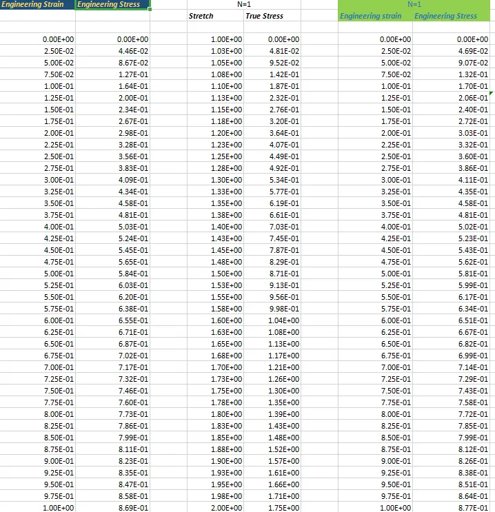
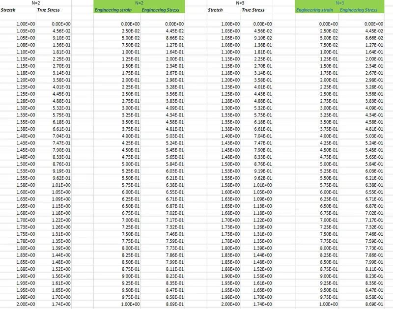
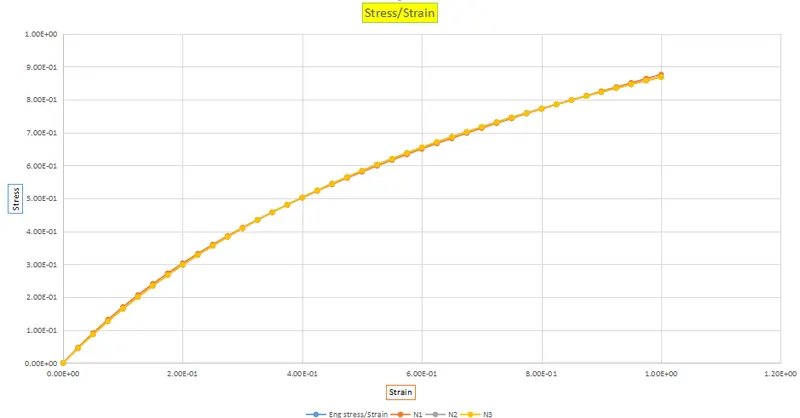
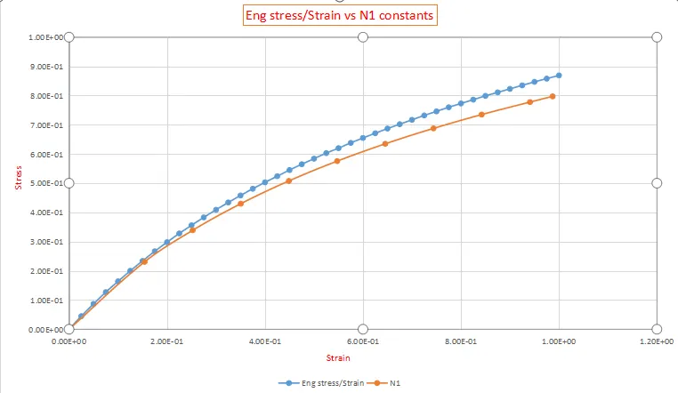
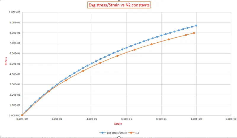
As we can see all the Constant values obtained from the d3hsp file is fitting with the Original Data

So from this, we can conclude all the Constants will Give similar results in compared with the original data

Material Validation:-

Change N=0 in the Material card and input the Mooney Rivlin Constants Individually Obtained from N=1, N=2, N=3 and validate

Constants from N=1 Constants From N=2:

Constants From N=3:-

Save the Keyword And Run the Simulation

The Simulation is Done Individually with The Constants Obtained from N=1, N=2, N=3

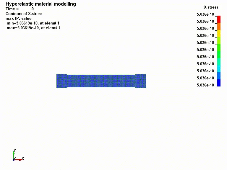
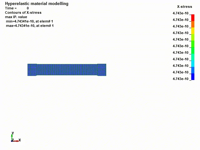
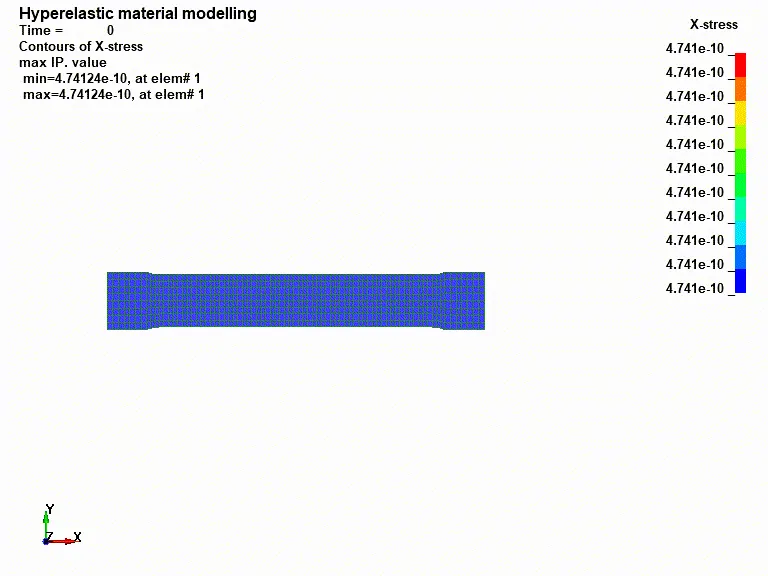
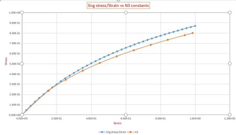
True Stress vs True Strain plotted from An Element From each Simulation

The True Stress and Strain Values Obtained from the Element is Converted to Engineering Stress/ strain

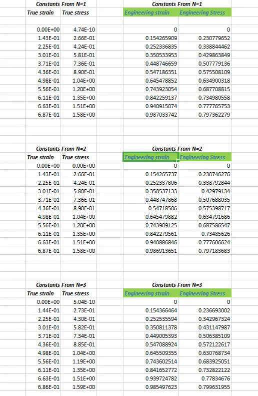
The Constants From N=1,2,3 are plotted with original Data

Ogden Material Model:-

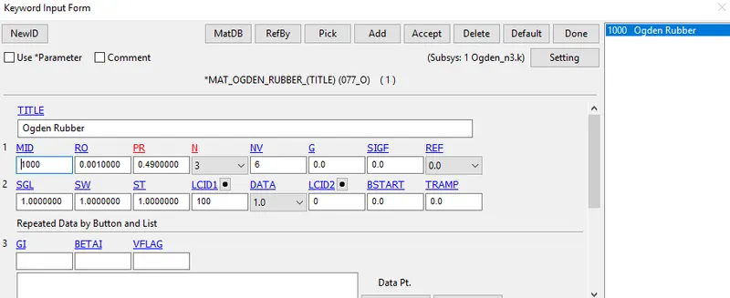
In this case, MAT_77_O_Ogden Rubber is Replaced instead of Hyperelastic Rubber

The Mat Ogden Card is Defined with the Properties of rubber

Density=0.001 gm/mm^3

Poissons Ratio=0.49

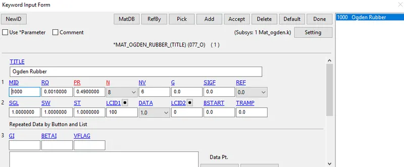
MAT_77_O_Ogden Rubber has the Property N in which same as Mat_Hyperelastic rubber where N can be defined from N=1 to N=8

Since it has 8 polynomials it can be defined better adjustment to the experimental data

The same Procedure is Repeated with N=3, N=6, N=8 Constants randomly and their Fit is analyzed with the Original data

For N=8,6,3

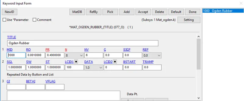
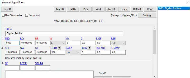
For N=8;8 Order polynomial values of alpha and beta are obtained and For 6 and 3- the same 6 and 3 order polynomial values of alpha and Beta will be acquired

N=8 N=6 N=3

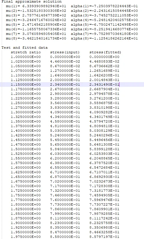
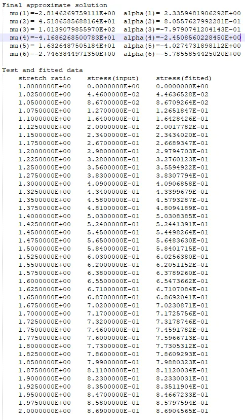
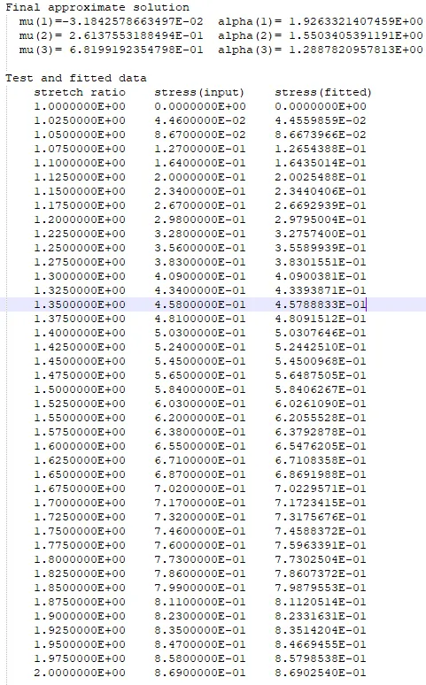
From The d3hsp file N values with Curve, the fit is obtained

The Curve fit is expressed in Stretch and Engineering Stress values, The Stretch is Converted into engineering Strain

The Curve Fit values are plotted with The original data to find the Best Fit

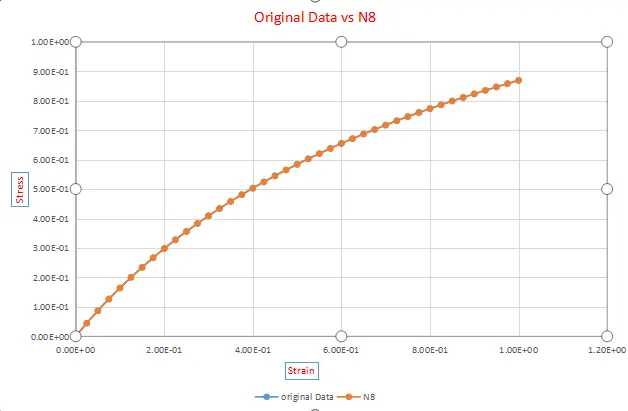
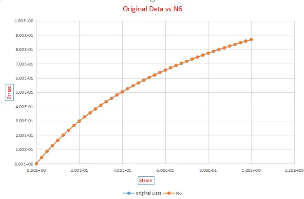
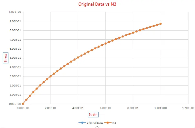
From the Plots, it's evident that N=8,6,3 polynomials Give the best and similar fit with the Original engineering stress / Strain data

Material Validation:-

Change N=0 in the Material card and input the Ogden Constants Individually Obtained from N=8, N=6, N=3 and validate

N=8 constants N=6 constants

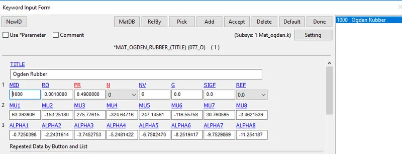
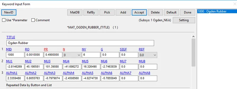
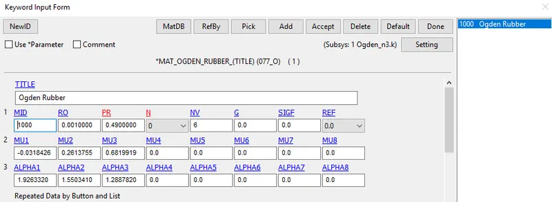
All other Control cards, boundary conditions, remains Unchanged

Save the Keyword And Run the Simulation

The Simulation is Done Individually with The Constants Obtained from N=8, N=6, N=3

N-8 N-6

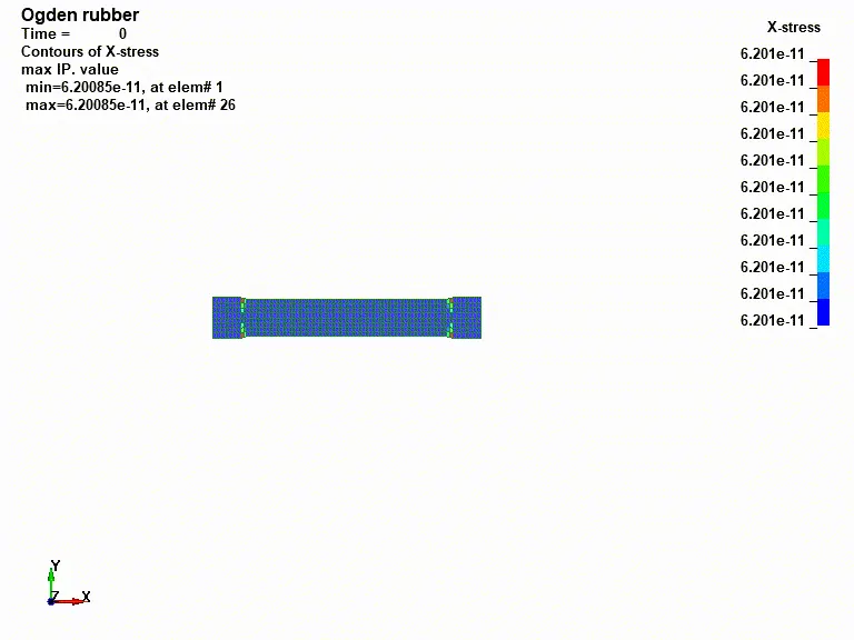
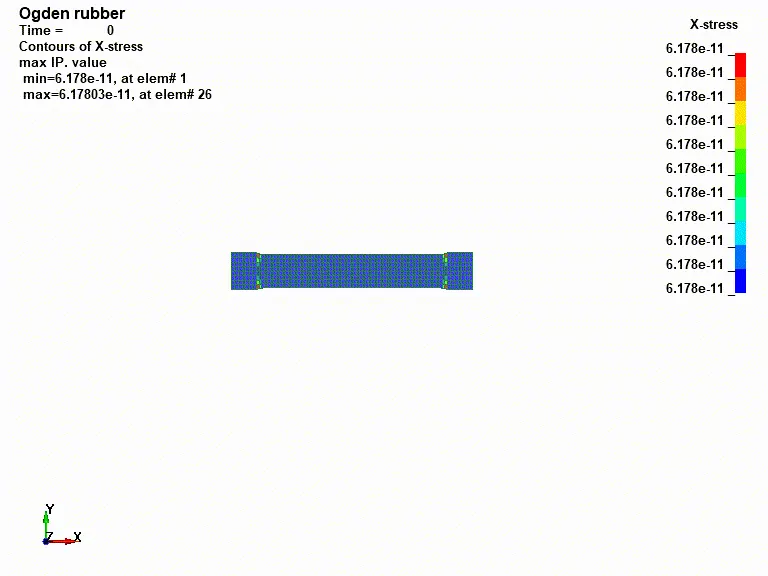
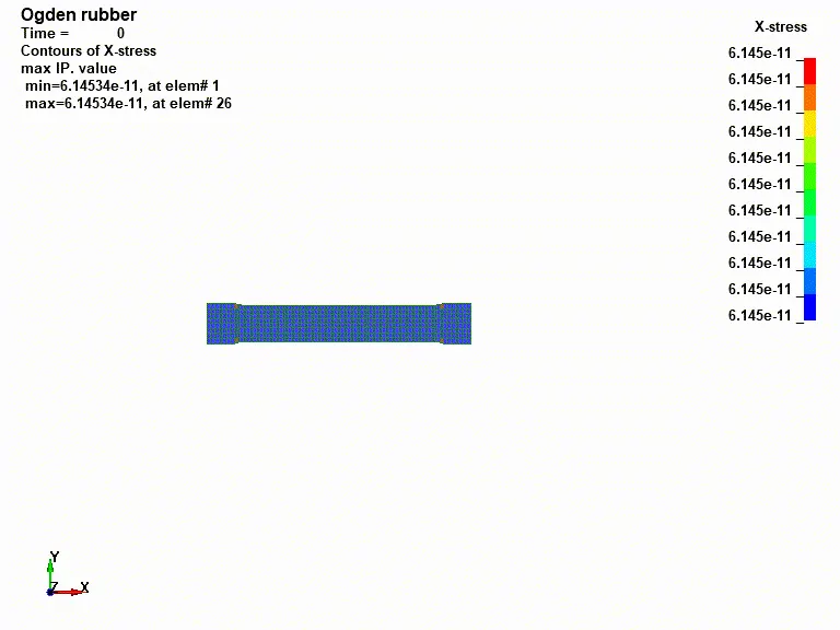
True Stress vs True Strain plotted from An Element From each Simulation

The True Stress and Strain Values Obtained from the Element is Converted to Engineering Stress/ strain

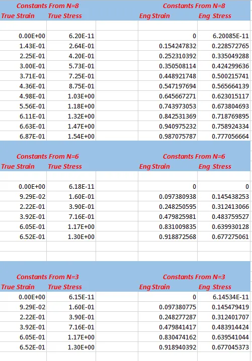
The Constants From N=8,6,3 are plotted with original Data

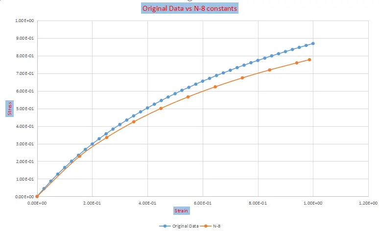
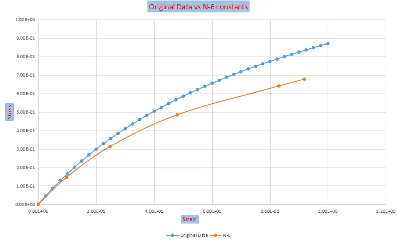
From the Graph the Fit values from N=8 Quite similar to the Original data and comparatively fits better than the constants from N=6 and N=3

Results:-

S.No	Material	Original cross-section	cross-section after Tensile Test	% Reduction
1	Hyperelastic Rubber	20	14.65	26.25%
2	Ogden	20	14.75	26.35%

1. From the result we can see that Odgen material is compressed quite more compared with the Hyperelastic in this simulation

2. both materials exhibit almost similar Properties

3. Hyperelastic material gives the most accurate fit In comparison with the Ogden material and the fit is almost constant for all parameters

4. whereas in Ogden The Fit constants of N=8 gives Quiet a similar fit with the original data

5. The Results Obtained may change in accordance with Poisson's ratio

6. The Ogden material has More polynomials ranging from 1-8 which is easy to use and model and gives better adjustment In defining with original data.