Week - 10 Hyperelastic Material Models

Skill-lync assignment 10

Aim: The objective of this assignment is to calculate the Mooney Rivlin and Ogden material constants from the given stress- strain data, use them in simulations of a dog-bone specimen and compare the results.

Case setup: The data provided is a set of engineering stress (MPa) & strain values up to a strain value of 1 (100%). The data is shown below.

Table 1: Input stress data

Engineering strain	Engineering stress (MPa)
0	0
0.025	4.46E-02
0.05	8.67E-02
0.075	1.27E-01
0.1	1.64E-01
0.125	2.00E-01
0.15	2.34E-01
0.175	2.67E-01
0.2	2.98E-01
0.225	3.28E-01
0.25	3.56E-01
0.275	3.83E-01
0.3	4.09E-01
0.325	4.34E-01
0.35	4.58E-01
0.375	4.81E-01
0.4	5.03E-01
0.425	5.24E-01
0.45	5.45E-01
0.475	5.65E-01
0.5	5.84E-01
0.525	6.03E-01
0.55	6.20E-01
0.575	6.38E-01
0.6	6.55E-01
0.625	6.71E-01
0.65	6.87E-01
0.675	7.02E-01
0.7	7.17E-01
0.725	7.32E-01
0.75	7.46E-01
0.775	7.60E-01
0.8	7.73E-01
0.825	7.86E-01
0.85	7.99E-01
0.875	8.11E-01
0.9	8.23E-01
0.925	8.35E-01
0.95	8.47E-01
0.975	8.58E-01
1	8.69E-01

Procedure: The data is worked on through the following set of steps.

1. The data provided is compiled into an excel spreadsheet and converted to the kg, mm, ms units.
2. A dog-bone specimen is then setup in the LS-PrePost workspace with adequate element formulation (ELFORM: 2) and a thickness of 5 mm.
3. The boundary conditions are setup such that one end of the component is fixed and the other is prescribed a displacement of 145 mm (100% strain) over a time period of 200 ms.
4. The MAT77_H-HYPERELASTIC_RUBBER material card is added to the component with N=1 so that constants C1 & C2 are solved for in the simulation. The material data curve is added from the spreadsheet. The density is set as 10^-6 kg/mm³ and Poisson’s ratio is set as 0.499999.
5. The model is setup for implicit analysis with an initial time step of 1 ms and a run time of 200 ms.
6. The keyword file is then saved and run using the LS-Run solver.
7. The effective stress vs. strain curve is plotted and output as an excel spreadsheet.
8. The d3hsp file is referred to for the values of the Mooney constants and those values are noted & recorded.
9. A copy of the keyword file is made and edited so that N is set as 2, so that constants C10, C01, C11, C20 and C02 are solved for. This modified file is then run and the relevant stress vs. strain curve is obtained.
10. The d3hsp file is referred to for the values of the hyper-elastic constants.
11. In a second copy of the keyword file, the value of N is set as 3 so that constants C10, C01, C11, C20, C02 and C30 are solved for. The modified file is then run and the stress vs. strain curve is obtained.
12. The d3hsp file is referred to for the value of the hyper-elastic constants.
13. The stress vs. strain curves for the three iterations are compared with the original data provided. The constants for the curve that is the closest match to the original data is chosen for a fourth copy of the first keyword file where the values of these constants are manually added to the material card.
14. This file is then run and the stress vs. strain curve is obtained. This curve is verified to match the original data and the curve from the respective iteration.

Result: The values for the various constants in the three iterations are compiled in the table below.

Table 2: Mooney Rivlin and Ogden constants

N	1	2	3
C10	1.768 X 10-4	2.595 X 10-4	2.611 X 10-4
c01	1.474 X 10-4	4.594 X 10-5	4.420 X 10-5
c11	0	-2.092 X 10-5	-6.077 X 10-6
c20	0	2.914 X 10-6	-2.666 X 10-6
c02	0	1.017 X 10-6	-9.966 X 10-6
c30	0		1.565 X 10-7

The stress vs. strain curves for the three iterations and the original data are illustrated below.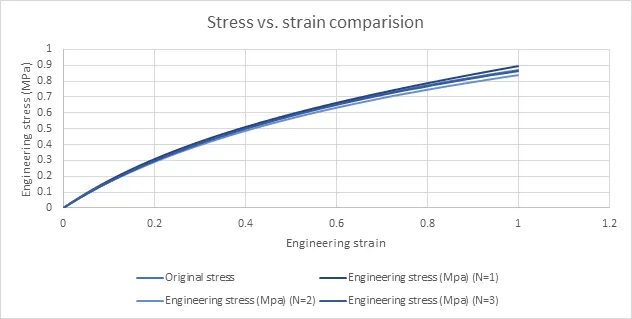

Figure 1: Stress vs. strain curves for different N values

It shows that the curve for N=3 best matches the original curve for the provided stress data. The final curve for iteration with N=0 is shown below along with the original curve and the curve for N=3.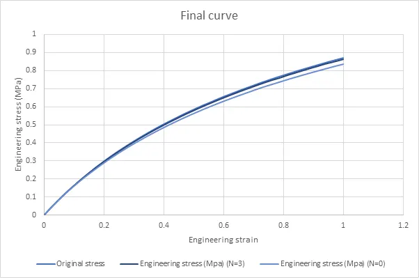

Figure 2: Final stress vs. strain curve with N=0

It shows that while the curve for N=0 does not match the original curve exactly, it is a near perfect replica of the curve for N=3, from which the Ogden material constants were selected for the final iteration.

Conclusion: The material constants for the given material were successfully computed from the stress data provided and used to replicate material behaviour through the use of MAT77 material card.